
This tutorial is part of a series illustrating basic concepts and techniques for machine learning in R. We will try to build a classifier of relapse in breast cancer. The analysis plan will follow the general pattern (simplified) of a recent paper.
This follows from: Machine learning for cancer classification - part 1 - preparing the data sets. This part covers how to build a Random Forest classification model to predict relapse in breast cancer from microarray expression data. We make the assumption that the data sets will be in the correct format as produced in part 1. The data sets in this tutorial are the 'training data' from the prior tutorial, retrieved from GSE2034. In a subsequent tutorial we will apply the classifier built here to the 'test data' (GSE2990) also downloaded in part 1. To avoid the hassle of Copy-Pasting every block of code, the full script can be downloaded here. But, first, let's review the basic principles of the Random Forests method.
Figure 1. A Random Forest is built one tree at a time.
A Random Forest is a collection of decision trees. Each tree gets a "vote" in classifying. There are two components of randomness involved in the building of a Random Forest. First, at the creation of each tree, a random subsample of the total data set is selected to grow the tree. Second, at each node of the tree, a well-performing gene from a random subset of all genes is chosen as a "splitter variable". The splitter variable attempts to separate patients in one class (e.g., Response) from those in the other class (e.g., Non-Response). The tree is grown with additional splitter variables until all terminal nodes (leaves) of the tree are purely one class or the other. This tree is then "tested" against the 1/3 of patients set aside, the "out of bag" (OOB) patients. Each OOB patient traverses the tree, going down one branch or another depending on his/her gene expression values for each splitter variable. These OOB patients are assigned a predicted class based on where they land in the tree (a vote). The entire process is repeated with new random divisions into 2/3 and 1/3 patient sets and new random gene sets for selection of splitter variables to produce additional trees and ultimately a forest. In each case a different subset of patients is used to build the tree and test its performance. At the end, each patient will have contributed to the construction of ~2/3 of all trees and been tested in the other ~1/3. Each "test" tree gives a vote for whether the patient will relapse or not relapse. The fraction of votes for relapse is an estimate of the probability of relapse and all patients will be predicted as either a relapse or non-relapse (using probability of 0.5 as the threshold). By comparing these predictions based on the OOB data to their known class, estimates of the accuracy of the overall forest can be obtained. The forest can then also be applied to independent test data or patients of unknown class (see next Figure 2).
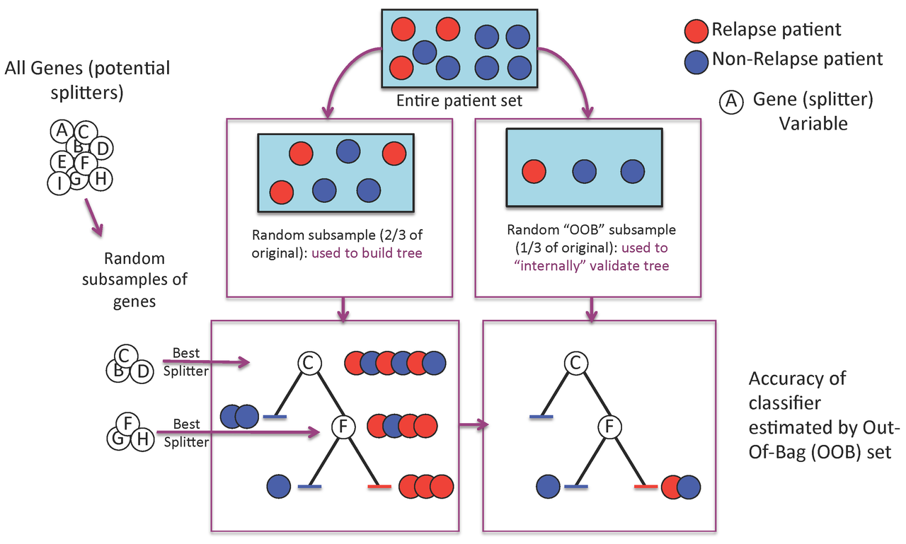
Figure 2. To predict new patients, each tree gets a vote...
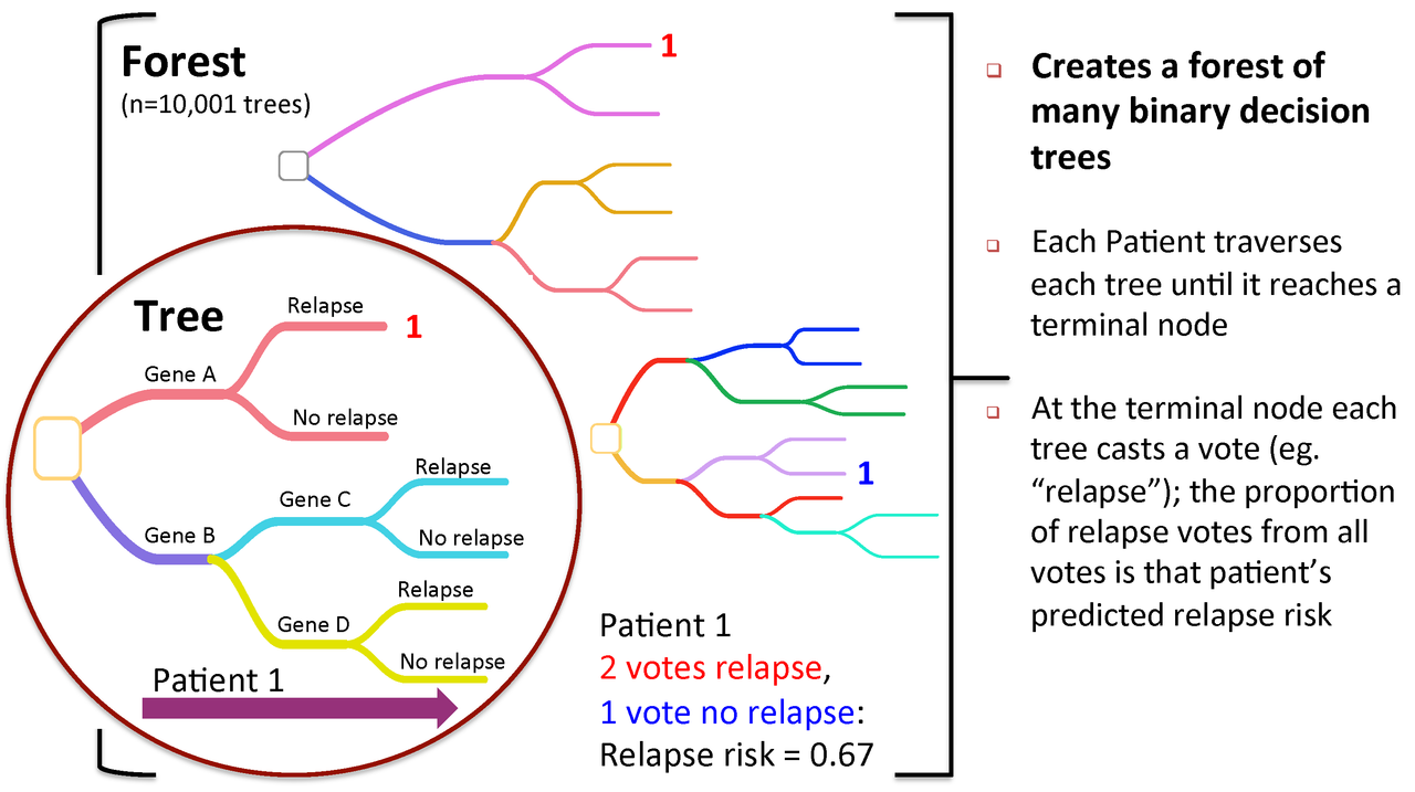
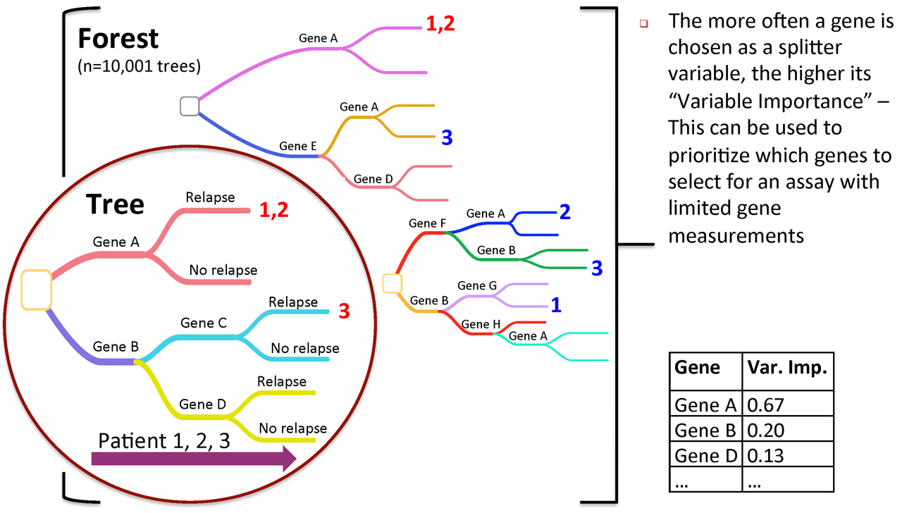
Figure 3. Variable importance is a feature of random forests
Now, let's proceed with the exercises. Install and load the necessary packages (if not already installed).
install.packages("randomForest")
install.packages("ROCR")
install.packages("Hmisc")
source("http://bioconductor.org/biocLite.R")
biocLite("genefilter")

library(randomForest)
library(ROCR)
library(genefilter)
library(Hmisc)
Set the working directory and file names for Input/output
setwd("/Users/ogriffit/git/biostar-tutorials/MachineLearning")
datafile="trainset_gcrma.txt"
clindatafile="trainset_clindetails.txt"
outfile="trainset_RFoutput.txt"
varimp_pdffile="trainset_varImps.pdf"
MDS_pdffile="trainset_MDS.pdf"
ROC_pdffile="trainset_ROC.pdf"
case_pred_outfile="trainset_CasePredictions.txt"
vote_dist_pdffile="trainset_vote_dist.pdf"
Next we will read in the data sets (expecting a tab-delimited file with header line and rownames). These were the outputs from the previous tutorial mentioned above. We also need to rearrange the clinical data so that it will be in the same order as the GCRMA expression data.
data_import=read.table(datafile, header = TRUE, na.strings = "NA", sep="\t")
clin_data_import=read.table(clindatafile, header = TRUE, na.strings = "NA", sep="\t")
clin_data_order=order(clin_data_import[,"GEO.asscession.number"])
clindata=clin_data_import[clin_data_order,]
data_order=order(colnames(data_import)[4:length(colnames(data_import))])+3 #Order data without first three columns, then add 3 to get correct index in original file
rawdata=data_import[,c(1:3,data_order)] #grab first three columns, and then remaining columns in order determined above
header=colnames(rawdata)
rawdata=rawdata[which(!is.na(rawdata[,3])),] #Remove rows with missing gene symbol
Next we filter out any variables (genes) that are not expressed or do not have enough variance to be informative in classification. We will first take the values and un-log2 them, then filter out any genes according to following criteria (recommended in multtest/MTP documentation): (1) At least 20% of samples should have raw intensity greater than 100; (2) The coefficient of variation (sd/mean) is between 0.7 and 10.
X=rawdata[,4:length(header)]
ffun=filterfun(pOverA(p = 0.2, A = 100), cv(a = 0.7, b = 10))
filt=genefilter(2^X,ffun)
filt_Data=rawdata[filt,]
We will assign the variables that pass this filtering process to a new data structure. Extract just the expression values from the filtered data and transpose the matrix. The latter is necessary because RandomForests expects the predictor variables (genes) to be represented as columns instead of rows. Finally, assign gene symbol as the predictor name.
#Get potential predictor variables
predictor_data=t(filt_Data[,4:length(header)])
predictor_names=c(as.vector(filt_Data[,3])) #gene symbol
colnames(predictor_data)=predictor_names
As a final step before the Random Forest classification, we have to set the variable we are trying to predict as our target variable. In this case, it is relapse status.
target= clindata[,"relapse..1.True."]
target[target==0]="NoRelapse"
target[target==1]="Relapse"
target=as.factor(target)
Finally we run the RF algorithm. NOTE: we use an ODD number for ntree. This is because when the forest/ensembl is used on test data, ties are broken randomly. Having an odd number of trees avoids this issue and makes the model fully deterministic. Also note, we will use down-sampling to attempt to compensate for unequal class-sizes (less relapses than non-relapses).
tmp = as.vector(table(target))
num_classes = length(tmp)
min_size = tmp[order(tmp,decreasing=FALSE)[1]]
sampsizes = rep(min_size,num_classes)
rf_output=randomForest(x=predictor_data, y=target, importance = TRUE, ntree = 10001, proximity=TRUE, sampsize=sampsizes, na.action = na.omit)
The final blocks of code produce various forms of output for analysis of the classifier, and final classification results. First, save the RF classifier with save(). This allows you to later load the saved model. This can be useful if you wish to rerun later parts of this script without the time-consuming model building. More importantly though it will allow you to apply the model you have built to new, independent samples for classification purposes.
save(rf_output, file="RF_model")
load("RF_model")
RandomForest calculates an importance measures for each variable. Let's save them to a new object for later use:
rf_importances=importance(rf_output, scale=FALSE)
The following lines will give an overview of the classifier's performance. Specifically, they will generate a confusion table to allow calculation of sensitivity, specificity, accuracy, etc.
confusion=rf_output$confusion
sensitivity=(confusion[2,2]/(confusion[2,2]+confusion[2,1]))*100
specificity=(confusion[1,1]/(confusion[1,1]+confusion[1,2]))*100
overall_error=rf_output$err.rate[length(rf_output$err.rate[,1]),1]*100
overall_accuracy=1-overall_error
class1_error=paste(rownames(confusion)[1]," error rate= ",confusion[1,3], sep="")
class2_error=paste(rownames(confusion)[2]," error rate= ",confusion[2,3], sep="")
overall_accuracy=100-overall_error
Next we will prepare each useful statistic for writing to an output file
sens_out=paste("sensitivity=",sensitivity, sep="")
spec_out=paste("specificity=",specificity, sep="")
err_out=paste("overall error rate=",overall_error,sep="")
acc_out=paste("overall accuracy=",overall_accuracy,sep="")
misclass_1=paste(confusion[1,2], rownames(confusion)[1],"misclassified as", colnames(confusion)[2], sep=" ")
misclass_2=paste(confusion[2,1], rownames(confusion)[2],"misclassified as", colnames(confusion)[1], sep=" ")
confusion_out=confusion[1:2,1:2]
confusion_out=cbind(rownames(confusion_out), confusion_out)
Finally, we print all of these to an output file. Note, we will be appending with multiple writes to the same file. This may generate a warning.
write.table(rf_importances[,4],file=outfile, sep="\t", quote=FALSE, col.names=FALSE)
write("confusion table", file=outfile, append=TRUE)
write.table(confusion_out,file=outfile, sep="\t", quote=FALSE, col.names=TRUE, row.names=FALSE, append=TRUE)
write(c(sens_out,spec_out,acc_out,err_out,class1_error,class2_error,misclass_1,misclass_2), file=outfile, append=TRUE)
For a simple visualization, we create a representation of the top 30 variables categorized by importance.
pdf(file=varimp_pdffile)
varImpPlot(rf_output, type=2, n.var=30, scale=FALSE, main="Variable Importance (Gini) for top 30 predictors")
dev.off()

An MDS plot provides a sense of the separation of classes.
pdf(file=MDS_pdffile)
target_labels=as.vector(target)
target_labels[target_labels=="NoRelapse"]="N"
target_labels[target_labels=="Relapse"]="R"
MDSplot(rf_output, target, k=2, xlab="", ylab="", pch=target_labels, palette=c("red", "blue"), main="MDS plot")
dev.off()

A common method of assessing a classifier's performance is to create an ROC curve and calculate the area under it (AUC). We use the relapse/non-relapse vote fractions as predictive variable. The ROC curve is generated by stepping through different thresholds for calling relapse vs non-relapse.
predictions=as.vector(rf_output$votes[,2])
pred=prediction(predictions,target)
#First calculate the AUC value
perf_AUC=performance(pred,"auc")
AUC=perf_AUC@y.values[[1]]
#Then, plot the actual ROC curve
perf_ROC=performance(pred,"tpr","fpr")
pdf(file=ROC_pdffile)
plot(perf_ROC, main="ROC plot")
text(0.5,0.5,paste("AUC = ",format(AUC, digits=5, scientific=FALSE)))
dev.off()

Produce a back-to-back histogram of vote distributions for Relapse and NoRelapse.
options(digits=2)
pdf(file=vote_dist_pdffile)
out <- histbackback(split(rf_output$votes[,"Relapse"], target), probability=FALSE, xlim=c(-50,50), main = 'Vote distributions for patients classified by RF', axes=TRUE, ylab="Fraction votes (Relapse)")
barplot(-out$left, col="red" , horiz=TRUE, space=0, add=TRUE, axes=FALSE)
barplot(out$right, col="blue", horiz=TRUE, space=0, add=TRUE, axes=FALSE)
dev.off()

Finally, we save our case predictions
case_predictions=cbind(clindata,target,rf_output$predicted,rf_output$votes)
write.table(case_predictions,file=case_pred_outfile, sep="\t", quote=FALSE, col.names=TRUE, row.names=FALSE)
After running this script you have generated a Random Forest Classifier of Relapse for breast cancer Affy data. Next, we will apply this classifier to the independent test data set. See Machine learning for cancer classification - part 3 - Predicting with a Random Forest Classifier. You also have a case_predictions file on which you can perform survival analysis, which will be the subject of a later tutorial. See Machine learning for cancer classification - part 4 - Plotting a Kaplan-Meier Curve for Survival Analysis.
Hello Mr Griffith,it was as absolute pleasure going through your tutorial(which btw is a rigorous introduction to ML applications using microarray data)!
I wanted to clarify something,can you please explain to me the meaning of the below mentioned code snippet and what its doing?
I got the
order()part but why the "without first three columns" and then adding 3 to get correct index?Same question for rawdata. Why consider the first 3 columns and then remaining in order as above?(I guess this part will be clear automatically if I understand the first part)
Thanks once again for this wonderful tutorial!
Please answer ASAP. Thanks for that too, in advance!
Shayantan
I'd avoid the "ASAP" part of the request - it's not really a good sign in forums.
@Ram I have my exams in a couple of days and hence the bad "sign" so to speak !!..Well now that you have gone through my question here,would you help by addressing the issue?
I still don't really get that part! Would love to hear from Mr Griffith though!
Hello,
The first three columns in the data set are non-numerical identifiers. We remove these to simplify the rest of the data-frame manipulations. Adding three to the index just makes sure gene order stays as intended.
Hope this helps!
Nick
I have a doubt, please correct me if I am wrong or missing anything. I found that, from the list of top 30 predictors, the gene "MLF1IP" is not present in the dataset GSE2034. As the list of predictors is generated from the original dataset only then how the above gene is not present in the dataset.
Dear Nicholas Spies,
I would like to ask some important questions regarding this specific part of the machine learning procedure with random forests in R, as I want to implement it to my current project. In detail, in contrast to the first part of the tutorial, my 2 datasets comprise of two colorectal cancer affymetrix datasets, but of different platform: hgu133a and hgu133plus2. Thus,
createDataPartition? Or it is irrelevant?Please excuse me for the disturbance or for any naive questions, but I'm using R for the last 7 months and this tutorial is very useful and crucial to implement in my analysis, in order to compare with some other methodologies I have implement regarding the selection of a subset of possible candidates-important genes(biomarkers for further validation), any help or advise on this matter would be grateful!
Efstathios-Iason
Can you clarify how best splitter (gene) is chosen in a random forest? Is it based on an expression threshold? If so, how is the threshold calculated?
Hi Nicolas,
I asked Obi the same question, but not sure who responds quicker. I have RNA-Seq data sets. How would I load them in to run Random forest? Would I need to use a completely different approach?
Many thanks
please ask this as a new question and not as an answer to this post.
Hi, first of all thanks for this tutorial, it's done very well. I have the following suggestione for the Random Forest statement :
With this addition I've solved the problems in the Part. 3 of this tutorial.
Thanks for the input! It's a great thought and I will add it to the example.