Entering edit mode

3.5 years ago
Hamid Ghaedi
3.2k
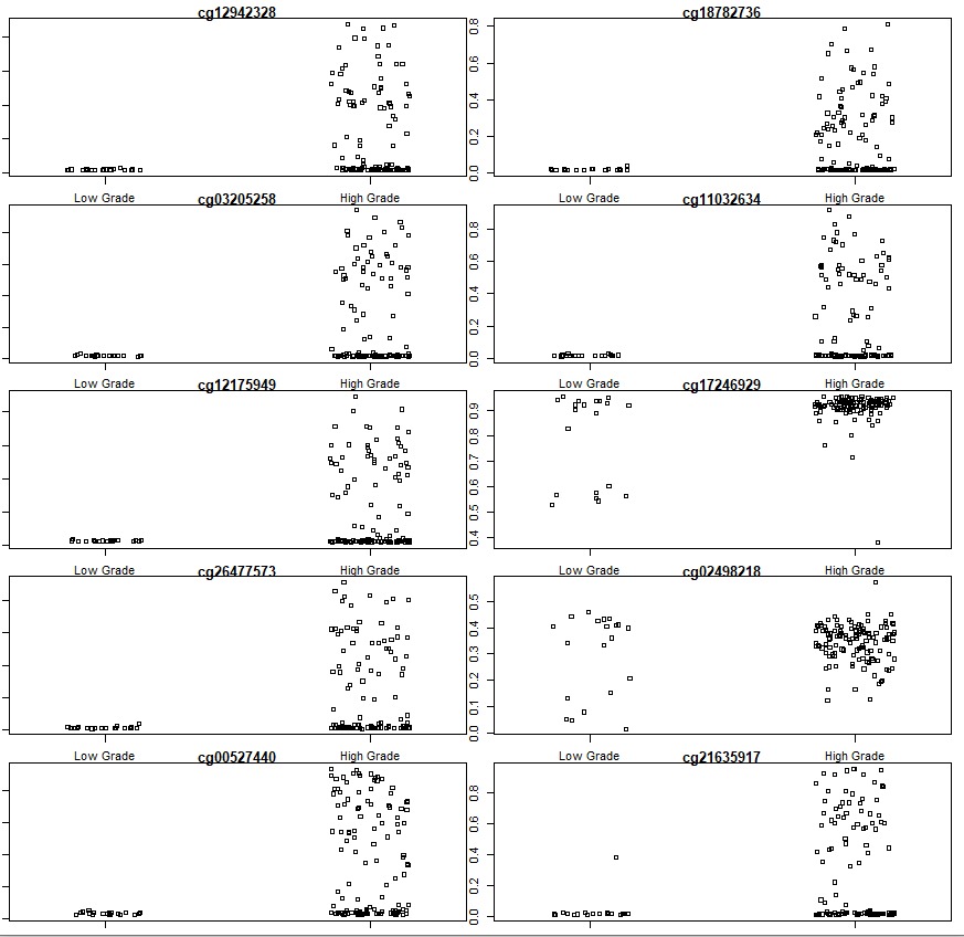
Differential variability analysis
Rather than testing for DMCs and DMRs, we may be interested in testing for differences between group variances. This could be quite helpful for feature selection in ML-based projects. In this situation, you may prefer to select variables that show great differences between groups.
#__________________________Differential variability_________________#
fitvar <- varFit(mval, design = design, coef = c(1,2))

# Summary of differential variability
summary(decideTests(fitvar))

topDV <- topVar(fitvar)
# Top 10 differentially variable CpGs between old vs. newborns
topDV

# visualization
# get beta values for ageing data
par(mfrow=c(5,2))
sapply(rownames(topDV)[1:10], function(cpg){
  plotCpg(bval, cpg=cpg, pheno= clinical$paper_Histologic.grade,
          ylab = "Beta values")
})


## if you got this error: Error in plot.new() : figure margins too large
#Do the following and try again:
#graphics.off()
#par("mar")
#par(mar=c(1,1,1,1))
Integrated analysis
###gene expression data download and analysis
## expression data
query.exp <- GDCquery(project = "TCGA-BLCA",
platform = "Illumina HiSeq",
data.category = "Gene expression",
data.type = "Gene expression quantification",
file.type = "results",
legacy = TRUE)
GDCdownload(query.exp, method = "api")
dat<- GDCprepare(query = query.exp, save = TRUE, save.filename = "blcaExp.rda")
rna <-assay(dat)
clinical.exp = data.frame(colData(dat))
# find what we have for grade
table(clinical.exp$paper_Histologic.grade)
#High Grade Low Grade ND
#384 21 3
table(clinical.exp$paper_Histologic.grade, clinical.exp$paper_mRNA.cluster)
# Get rid of ND and NA samples, normal samples
clinical.exp <- clinical.exp[(clinical.exp$paper_Histologic.grade == "High Grade" |
clinical.exp$paper_Histologic.grade == "Low Grade"), ]
clinical.exp$paper_Histologic.grade[clinical.exp$paper_Histologic.grade == "High Grade"] <- "High_Grade"
clinical.exp$paper_Histologic.grade[clinical.exp$paper_Histologic.grade == "Low Grade"] <- "Low_Grade"
# since most of low-graded are in Luminal_papilary category, we remain focus on this type
clinical.exp <- clinical.exp[clinical.exp$paper_mRNA.cluster == "Luminal_papillary", ]
clinical.exp <- clinical.exp[!is.na(clinical.exp$paper_Histologic.grade), ]
# keep samples matched between clinical.exp file and expression matrix
rna <- rna[, row.names(clinical.exp)]
all(rownames(clinical.exp) %in% colnames(rna))
#TRUE
## A pipeline for normalization and gene expression analysis (edgeR and limma)
edgeR_limma.pipe = function(
exp_mat,
groups,
ref.group=NULL){
group = factor(clinical.exp[, groups])
if(!is.null(ref.group)){group = relevel(group, ref=ref.group)}
# making DGEList object
d = DGEList(counts= exp_mat,
samples=clinical.exp,
genes=data.frame(rownames(exp_mat)))
# design
design = model.matrix(~ group)
# filtering
keep = filterByExpr(d,design)
d = d[keep,,keep.lib.sizes=FALSE]
rm(keep)
# Calculate normalization factors to scale the raw library sizes (TMM and voom)
design = model.matrix(~ group)
d = calcNormFactors(d, method="TMM")
v = voom(d, design, plot=TRUE)
# Model fitting and DE calculation
fit = lmFit(v, design)
fit = eBayes(fit)
# DE genes
DE = topTable(fit, coef=ncol(design), sort.by="p",number = nrow(rna), adjust.method = "BY")
return(
list(
DE=DE, # DEgenes
voomObj=v, # NOrmalized counts
fit=fit # DE stats
)
)
}
# Runing the pipe
de.list <- edgeR_limma.pipe(rna,"paper_Histologic.grade", "Low_Grade" )
de.genes <- de.list$DE
#ordering diffrentially expressed genes
de.genes<-de.genes[with(de.genes, order(abs(logFC), adj.P.Val, decreasing = TRUE)), ]
# voomObj is normalized expression values on the log2 scale
norm.count <- data.frame(de.list$voomObj)
norm.count <- norm.count[,-1]
norm.count <- t(apply(norm.count,1, function(x){2^x}))
colnames(norm.count) <- chartr(".", "-", colnames(norm.count))
#______________preparing methylation data for cis-regulatory analysis____________#
# finding probes in promoter of genes
table(data.frame(ann450k)$Regulatory_Feature_Group) ## to find regulatory features of probes
# selecting a subset of probes associated with promoters
promoter.probe <- rownames(data.frame(ann450k))[data.frame(ann450k)$Regulatory_Feature_Group
%in% c("Promoter_Associated", "Promoter_Associated_Cell_type_specific")]
# find genes probes with significantly different methylation statuses in
# low- and high-grade bladder cancer
low.g_id <- clinical$barcode[clinical$paper_Histologic.grade == "Low Grade"]
high.g_id <- clinical$barcode[clinical$paper_Histologic.grade == "High Grade"]
dbet <- data.frame (low.grade = rowMeans(bval[, low.g_id]),
high.grade = rowMeans(bval[, high.g_id]))
dbet$delta <- abs(dbet$low.grade - dbet$high.grade)
db.probe <- rownames(dbet)[dbet$delta > 0.2] # those with deltabeta > 0.2
db.probe <- db.probe %in% promoter.probe # those resided in promoter
# those genes flanked to promote probe
db.genes <- data.frame(ann450k)[rownames(data.frame(ann450k)) %in% db.probe, ]
db.genes <- db.genes[, c("Name","UCSC_RefGene_Name")]
db.genes <- tidyr::separate_rows(db.genes, Name, UCSC_RefGene_Name) # extending collapsed cells
db.genes$comb <- paste(db.genes$Name,db.genes$UCSC_RefGene_Name) # remove duplicates
db.genes <- db.genes[!duplicated(db.genes$comb), ]
db.genes <- db.genes[, -3]
# polishing matrices to have only high grade samples
cis.bval.mat <- bval[, high.g_id]
cis.exp.mat <- norm.count[, rownames(clinical.exp)[clinical.exp$paper_Histologic.grade == "High_Grade"]]
#making patient name similar
colnames(cis.bval.mat) <- substr(colnames(cis.bval.mat),1,19)
colnames(cis.exp.mat) <- substr(colnames(cis.exp.mat),1,19)
cis.exp.mat <- cis.exp.mat[, colnames(cis.bval.mat)]
#editing expression matrix rowname
df <- data.frame(name = row.names(cis.exp.mat)) # keeping rownames as a temporary data frame
df <- data.frame(do.call('rbind', strsplit(as.character(df$name),'|',fixed=TRUE)))
rowName <- df$X1
# find duplicates in rowName, if any
table(duplicated(rowName))
#FALSE TRUE
#20530 1
# in order to resolve duplucation issue
rowName[duplicated(rowName) == TRUE]
#[1] "SLC35E2"
#
rowName[grep("SLC35E2", rowName)[2]] <- "SLC35E2_2"
#setting rna row names
row.names(cis.exp.mat) <- rowName
rm(df, rowName) # removing datasets that we do not need anymore
#__________________correlation analysis__________________#
cis.reg = data.frame( gene=character(0), cpg=character(0), pval=numeric(0), cor=numeric(0))
for (i in 1:nrow(db.genes)){
cpg = db.genes[i,][7]
gene = db.genes[i,][8]
if (gene %in% rownames(cis.exp.mat)){
df1 <- data.frame(exp= cis.exp.mat[as.character(gene), ])
df2 <- t(cis.bval.mat[as.character(cpg), ])
df <- merge(df1,df2, by = 0)
res <- cor.test(df[,2], df[,3], method = "pearson")
pval = round(res$p.value, 4)
cor = round(res$estimate, 4)
cis.reg[i,] <- c(gene, cpg, pval, cor)
}
}
cis.reg$adj.P.Val = round(p.adjust(cis.reg$pval, "fdr"),4)
cis.reg <- cis.reg[with(cis.reg, order(cor, adj.P.Val)), ]
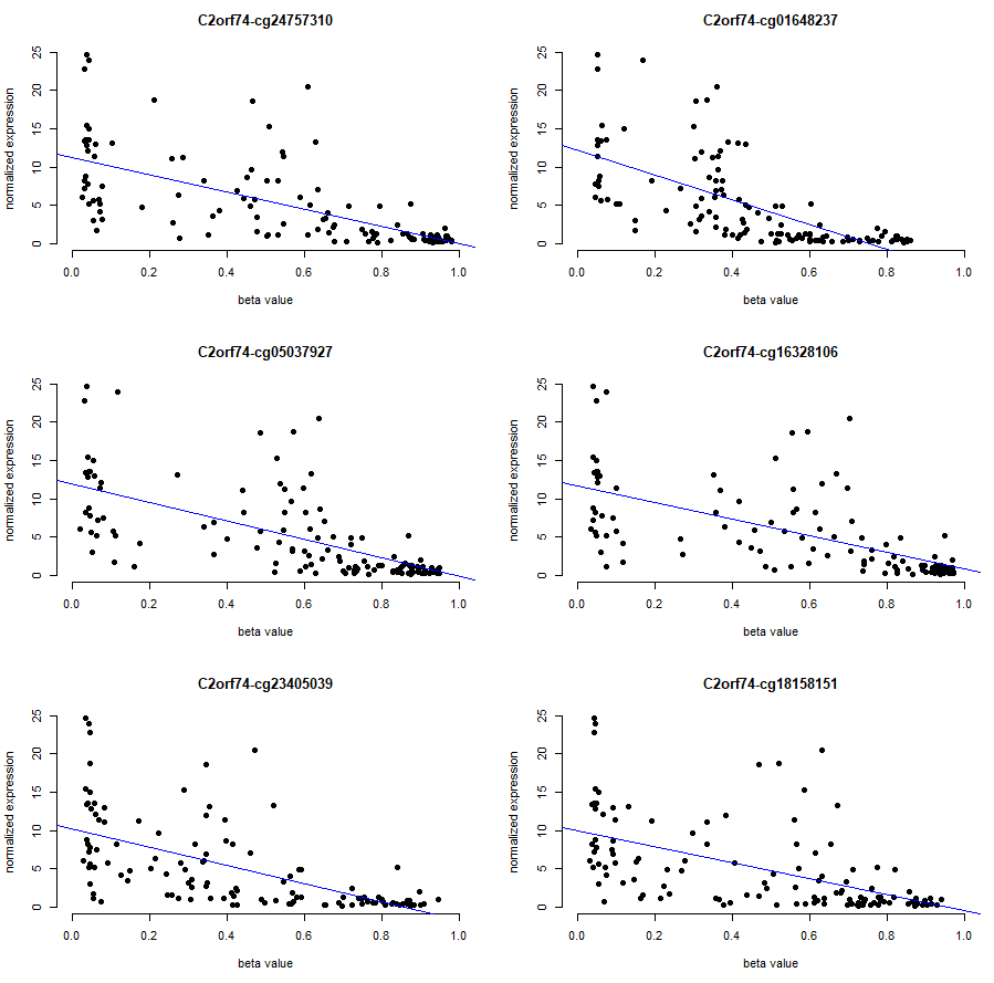
# top pair visualization
# inspecting the results, C2orf74 gene has a significant correlation with probes:
gen.vis <- merge(data.frame(exp= cis.exp.mat["C2orf74", ]),
t(cis.bval.mat[c("cg24757310", "cg01648237", "cg05037927", "cg16328106", "cg23405039", "cg18158151"), ]),
by = 0)
par(mfrow=c(3,2))
sapply(names(gen.vis)[3:8], function(cpg){
plot(x= gen.vis[ ,cpg], y = gen.vis[,2], xlab = "beta value",
xlim = c(0,1),
ylab = "normalized expression" ,
pch = 19,
main = paste("C2orf74",cpg, sep = "-"),
frame = FALSE)
abline(lm(gen.vis[,2] ~ gen.vis[ ,cpg], data = gen.vis), col = "blue")
})
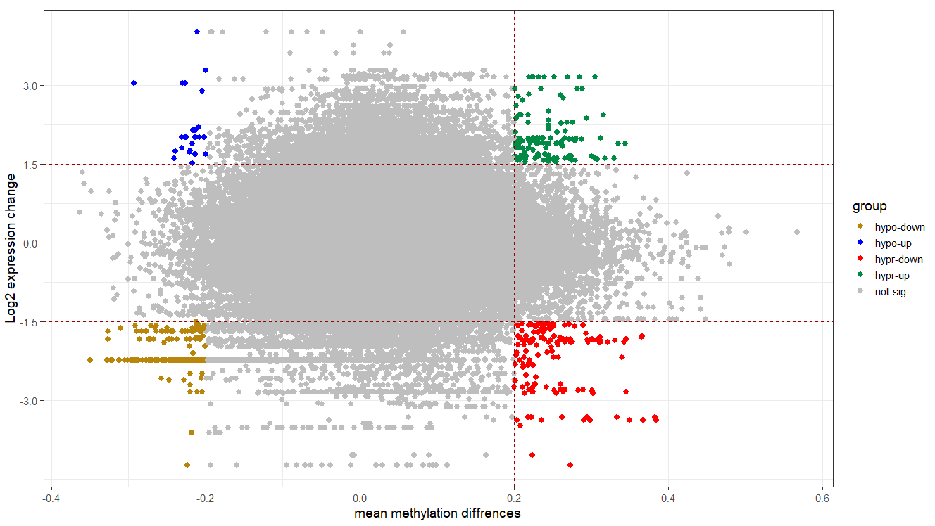
Starburst plot for trans-regulation visualization
# adding genes to delta beta data
tran.reg <- data.frame(ann450k)[rownames(data.frame(ann450k)) %in% rownames(dbet), ][, c(4,24)]
tran.reg <- tidyr::separate_rows(tran.reg, Name, UCSC_RefGene_Name) # extending collapsed cells
tran.reg$comb <- paste(tran.reg$Name,tran.reg$UCSC_RefGene_Name) # remove duplicates
tran.reg <- tran.reg[!duplicated(tran.reg$comb), ]
tran.reg <- tran.reg[, -3]
names(tran.reg)[2] <- "gene"

# merging with deltabeta dataframe
dbet$Name <- rownames(dbet)
tran.reg <- merge(tran.reg, dbet, by = "Name")
# joining with differential expression analysis result
#editing expression matrix rowname
df <- data.frame(name = row.names(de.genes)) # keeping rownames as a temporary data frame
df <- data.frame(do.call('rbind', strsplit(as.character(df$name),'|',fixed=TRUE)))
df$X1[df$X1 == "?"] <- df$X2 # replace "? with entrez gene number
rowName <- df$X1
# find duplicates in rowName, if any
table(duplicated(rowName))
#FALSE  TRUE
#16339     1
# in order to resolve  duplication issue
rowName[duplicated(rowName) == TRUE]
grep("SLC35E2", rowName)
#[1]  9225 15546
rowName[15546] <- "SLC35E2_2"
#setting rna row names
row.names(de.genes) <- rowName
rm(df, rowName) # removing datasets that we do not need anymore
de.genes$rownames.exp_mat. <- rownames(de.genes)
names(de.genes)[1] <- "gene"
# merging
tran.reg <- merge(tran.reg, de.genes, by = "gene")
# inspecting data
hist(tran.reg$logFC)
hist(tran.reg$delta) # delta was calculated as abs(delta), re-calculate to have original value
tran.reg$delta <- tran.reg$high.grade - tran.reg$low.grade

# defining a column for coloring
tran.reg$group <- ifelse(tran.reg$delta <= -0.2 & tran.reg$logFC <= -1.5, "hypo-down",
                       ifelse(tran.reg$delta <= -0.2 & tran.reg$logFC >= 1.5, "hypo-up",
                              ifelse(tran.reg$delta >= 0.2 & tran.reg$logFC <= -1.5, "hypr-down",
                                     ifelse(tran.reg$delta >= 0.2 & tran.reg$logFC >= 1.5, "hypr-up", "not-sig"))))

# plotting
cols <- c("hypo-down" = "#B8860B", "hypo-up" = "blue", "not-sig" = "grey", "hypr-down" = "red", "hypr-up" = "springgreen4")

ggplot(tran.reg, aes(x = delta, y = logFC, color = group)) +
  geom_point(size = 2.5, alpha = 1, na.rm = T) +
  scale_colour_manual(values = cols) +
  theme_bw(base_size = 14) +
  geom_hline(yintercept = 1.5, colour="#990000", linetype="dashed") +
  geom_hline(yintercept = -1.5, colour="#990000", linetype="dashed") +
  geom_vline(xintercept = 0.2, colour="#990000", linetype="dashed") +
  geom_vline(xintercept = -0.2, colour="#990000", linetype="dashed") +
  xlab("mean methylation diffrences") +
  ylab("Log2 expression change")
References:
1- A cross-package Bioconductor workflow for analyzing methylation array data
Hello Professor, how did you find the probes in the promoter region? Do you screen the probes based on the UCSC_RefGene_Group image (5'UTR; TSS1500; TSS200, etc.) in the comment information?
Here is how I did that part .
As you may see in the code I asked to have probes that have
"Promoter_Associated"or"Promoter_Associated_Cell_type_specific"value underRegulatory_Feature_Groupcolumn inann450kobject.Hello!
I am performing your 'cis.reg' correlation analysis but I am facing some troubles: I have several NA values in my cis.reg dataframe. Can you please enlighten me on to why?
Here is my detailed data:
Many thanks in advance!!