
Clustering is a data mining method to identify unknown possible groups of items solely based on intrinsic features and no external variables. Basically, clustering includes four steps:
1) Data preparation and Feature selection,
2) Dissimilarity matrix calculation,
3) applying clustering algorithms,
4) Assessing cluster assignment
I use an RNA-seq dataset on 476 patients with non-muscle invasive bladder cancer. To make this tutorial reproducible, clinical data can be downloaded from GitHub and normalized RNA-seq data can be obtained through this link. So if you like to use these materials, start your analysis from the 'feature selection' section onward. Also, the GitHub repo could provide more details on each step of the analysis.
Data preparation and Feature selection
In this step, we need to: filter out incomplete cases and low expressed genes, deal with missing values (removing or value imputation), and then transform/normalize gene expression values.
In the dataset, there is no missing value. For transformation/normalization, I use variance stabilizing transformation (VST) implemented as vst function from DESeq2 packages which at the same time will normalize the raw count also. Using other types of transformation like Z score, log transformation is also common. If the expression matrix contains estimated transcript counts (like RSEM) or counts normalized for sequencing depth (like FPKM) , log2 transformation of the values would prepare the data for clustering.
Feature selection: A feature selection could be helpful to limit the analysis to those genes that possibly explain variation between samples in the cohort. I select 2k, 4k, and 6k top genes based on median absolute deviation (MAD). A number of other approaches like feature selection based on the most variance, feature dimension reduction and extraction based on Principal Component Analysis (PCA), and feature selection based on the Cox regression model could be applied.
#_________________________________reading data and processing_________________________________#
# reading count data
rna <- read.table("Uromol1_CountData.v1.csv", header = T, sep = ",", row.names = 1)

dim(rna)
# [1] 60483   476  this is a typical output from hts-seq count matrix with more than 60,000 genes

# dissecting dataset based on gene-type
library(biomaRt)
mart <- useDataset("hsapiens_gene_ensembl", useMart("ensembl"))
genes <- getBM(attributes= c("ensembl_gene_id","hgnc_symbol", "gene_biotype"),
               mart= mart)

# see gene types returned by biomaRt
data.frame(table(genes$gene_biotype))[order(- data.frame(table(genes$gene_biotype))[,2]), ]

# we will continue with protein coding here:
rna <- rna[substr(rownames(rna),1,15) %in% genes$ensembl_gene_id[genes$gene_biotype == "protein_coding"],]

dim(rna)
#[1] 19581   476 These are protein coding genes

# reading associated clinical data
clinical.exp <- read.table("uromol_clinic.csv", sep = ",", header = T, row.names = 1)

# making sure about sample order in rna and clincal.exp dataset
all(rownames(clinical.exp) %in% colnames(rna))
#[1] TRUE
all(rownames(clinical.exp) == colnames(rna))
#[1] FALSE
# reordering rna dataset
rna <- rna[, rownames(clinical.exp)]
#______________________ Data tranformation & Normalization ______________________________#
library(DESeq2)
dds <- DESeqDataSetFromMatrix(countData = rna,
                              colData = clinical.exp,
                              design = ~ 1) # 1 passed to the function because of no model
# pre-filteration,
# Keeping genes with expression in 10% of samples with a count of 10 or higher
keep <- rowSums(counts(dds) >= 10) >= round(ncol(rna)*0.1)
dds <- dds[keep,]

# vst tranformation
vsd <- assay(vst(dds))
#_________________________________# Feature Selection _________________________________#
mads=apply(vsd,1,mad)
# check data distribution
#hist(mads, breaks=nrow(vsd)*0.1)
# selecting features
mad2k=vsd[rev(order(mads))[1:2000],]
#mad4k=vsd[rev(order(mads))[1:4000],]
#mad6k=vsd[rev(order(mads))[1:6000],]
Dissimilarity matrix calculation and clustering algorithms:
Dissimilarity matrix
There is a diverse list of dissimilarity matrix calculation methods (distance measures). To see a list of available distance measures please check ?stats::dist. For log-transformed gene expression, Euclidean-based measures can be applied. For RNA-seq normalized counts, correlation-based measures (Pearson, Spearman) or a Poisson-based distance can be used.
Clustering algorithms: The most widely used algorithms are partitional clustering and hierarchical clustering.
Partitional clustering is a clustering method used to classify samples into multiple clusters based on their similarity. The algorithms are required to specify the number of clusters to be generated. The commonly used partitional clustering includes K-means clustering (KM): each cluster is represented by the center or means of the data points belonging to the cluster. This method is sensitive to outliers.
In K-medoids clustering or PAM (Partitioning Around Medoids), each cluster is represented by one of the objects in the cluster. PAM is less sensitive to outliers.
In contrast to partitional clustering, hierarchical clustering (HC) does not require pre-specifying the number of clusters to be generated. To compute distances between clusters in HC, there are different ways to do cluster agglomeration (i.e, linkage ) like “ward.D”, “ward.D2”, “single”, “complete”, “average”, “mcquitty”, “median” or “centroid”. Generally, complete linkage and Ward’s method are preferred for gene expression analysis.
In practice, HC, KM, and PAM are commonly used for gene expression data.
It would be quite challenging to decide between several clusters and the membership of samples in each cluster.
To quantitatively address these two issues, I use Consensus Clustering (CC) approach. Applying this method has proved to be effective in new cancer subclass discoveries. For more information on the methodology please refer to the seminal paper by Monti et al. (2003) and the ConsensusClusterPlus package manual.
#________________________# Clustering & Cluster assignment validation __________________________#
# finding optimal clusters by CC
library(ConsensusClusterPlus)
results = ConsensusClusterPlus(mad2k, # normalized expression matrix
                               maxK=6, # maximum k to make clusters
                               reps=50, # resampling
                               pItem=0.8, # item resampling
                               pFeature=1, # gene resampling
                               title= "geneExp", # output title
                               clusterAlg="pam", # clustering algorithm
                               distance="spearman", # distance measure
                               seed=1262118388.71279, # random number
                               plot="pdf") # output file format
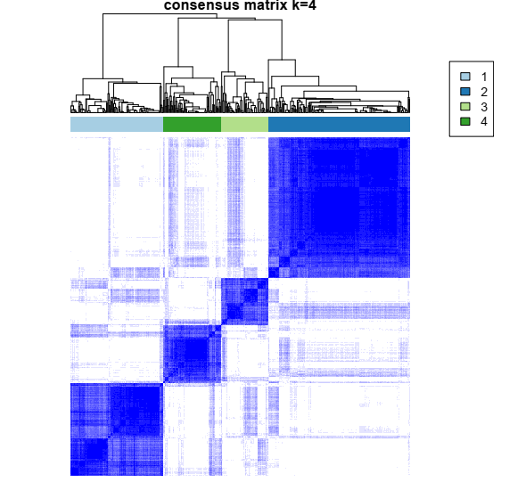
The above command returns several plots which are helpful in deciding on cluster number:
1- Color-coded heatmap corresponding to the consensus matrix that represents consensus values from 0–1; white corresponds to 0 (never clustered together) and dark blue to 1 (always clustered together). Here I only posted a heatmap for k = 4.
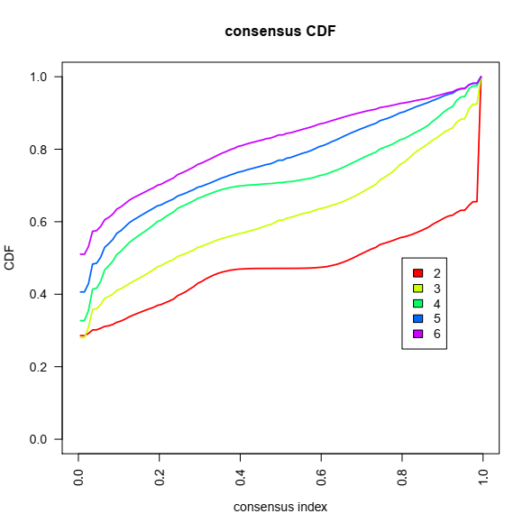
2- Consensus Cumulative Distribution Function (CDF) plot, This graphic lets one determine at what number of clusters,k, the CDF reaches an approximate maximum: here 4 or 5.
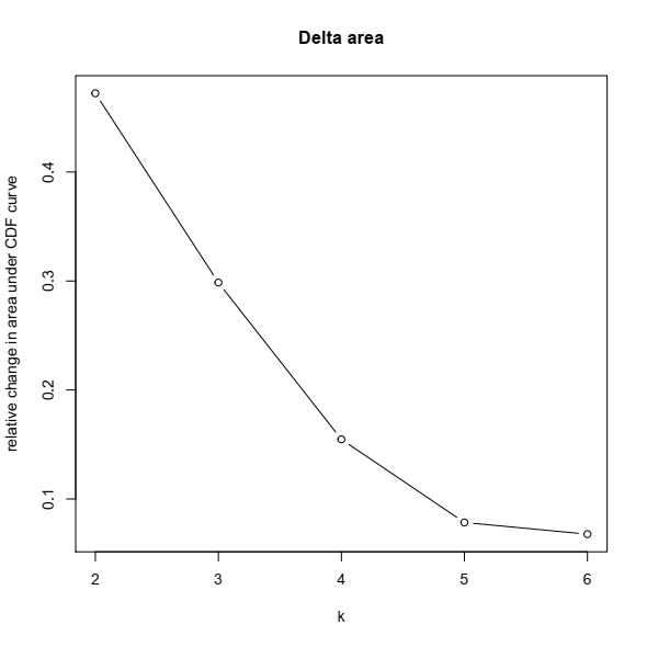
3- Based on the CDF plot, a chart for the relative change in area under the CDF curve can be plotted. This plot allows a user to determine the relative increase in consensus and determine the k at which there is no appreciable increase:
Assessing cluster assignment
This is the procedure of assessing the goodness of clustering results. Here I will use the Silhouette method for cluster assessment and survival analysis to see how technically and biologically the clusters that we defined make sense.
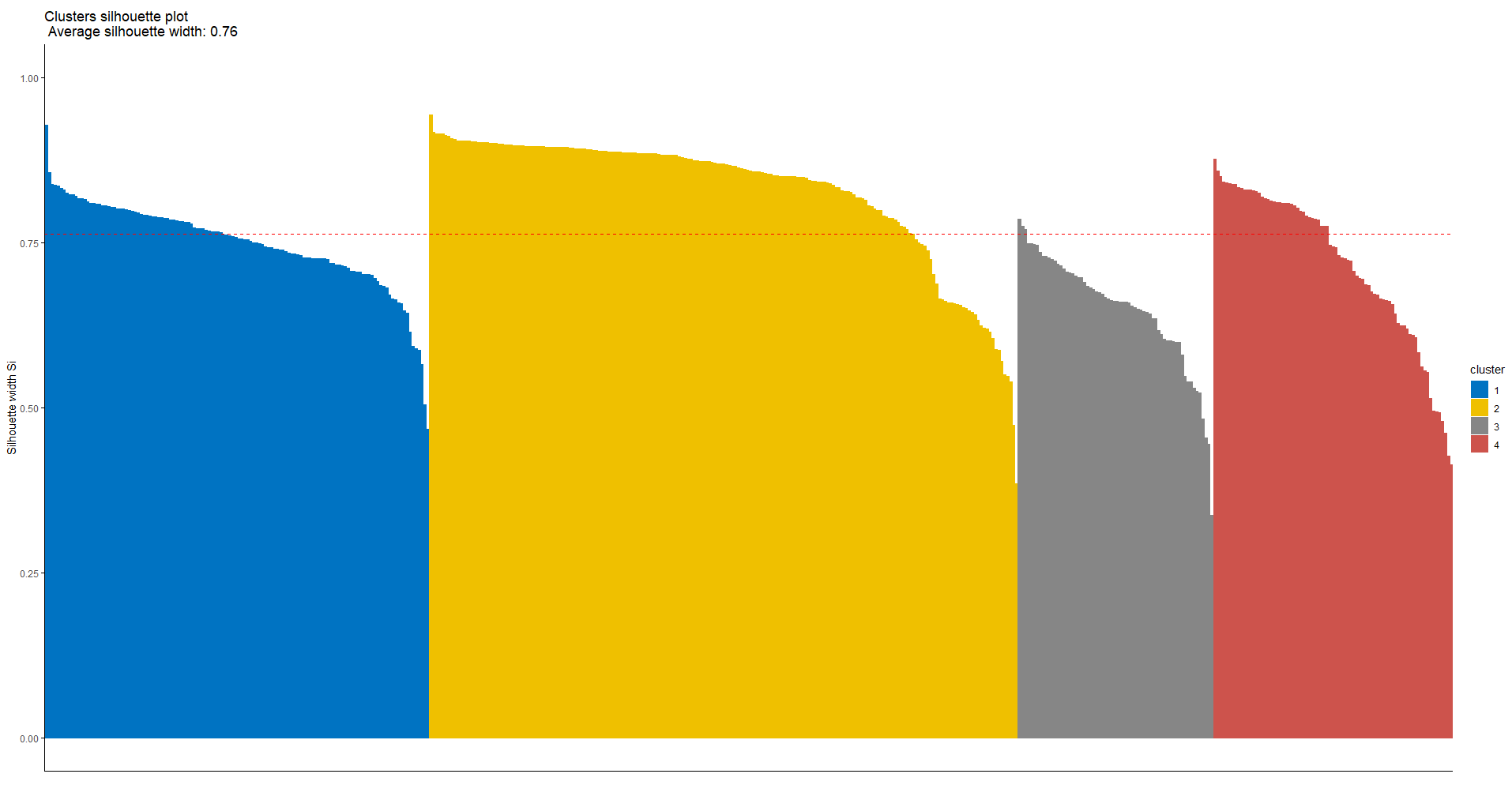
The silhouette method can be used to investigate the separation distance between the obtained clusters. The Silhouette plot reflects a measure of how close each data point in one cluster is to a point in the neighboring clusters. Silhouette width has a range of -1 to +1. A value near +1 shows that the sample is far away from the closest data point from the neighboring cluster. A negative value may indicate a wrong cluster assignment and a value close to 0 means an arbitrary cluster assignment to that data point.
#__________________________#Assessing cluster assignment ______________________________#
#Silhouette width analysis
cc4 = results[[4]]

# calcultaing Silhouette width using the cluster package
library(cluster)
cc4Sil = silhouette(x = cc4[[3]],
                    dist = as.matrix(1- cc4[[4]]))

#For visualization:
library(factoextra)
fviz_silhouette(cc4Sil, palette = "jco",
                 ggtheme = theme_classic())
```r

The above function returns a summary of the Silhouette width for each cluster:

```r
  cluster size ave.sil.width
1       1  130          0.75
2       2  199          0.83
3       3   66          0.65
4       4   81          0.72
Since by clustering, one should expect to find clusters of samples that are significantly different in terms of survival probability, I perform survival analysis between clusters (subtypes) to see significant differences, if any. As the result suggest it seems that clusters 2 and 4 have a significant difference in terms of survival probability from cluster 1:
#________________________#Assessing cluster assignment _________________________________#
#Survival analysis
### preparing dataset for survival analysis
cc4Class = data.frame(cc4$consensusClass)
cc4Class$ID = rownames(cc4Class)
cc4Class = data.frame(cc4Class[match(rownames(clinical.exp),cc4Class$ID),])
all(cc4Class$ID == rownames(clinical.exp))

# new encoding for status, time, and cluster
clinical.exp$status = ifelse(clinical.exp$Progression.to.T2. == "NO", 0,1)
clinical.exp$time = as.numeric(clinical.exp$Progression.free.survival..months. * 30)
clinical.exp$cluster = as.factor(cc4Class$cc4.consensusClass)

library(survival)

res.cox <- coxph(Surv(time, status) ~ cluster, data = clinical.exp)
res.cox

Call:
coxph(formula = Surv(time, status) ~ cluster, data = clinical.exp)

             coef exp(coef) se(coef)      z       p
cluster2 -1.47638   0.22846  0.48357 -3.053 0.00226
cluster3  0.22532   1.25272  0.42213  0.534 0.59351
cluster4 -2.39949   0.09076  1.03301 -2.323 0.02019

Likelihood ratio test=21.88  on 3 df, p=6.908e-05
n= 476, number of events= 31

summary(res.cox)

Call:
coxph(formula = Surv(time, status) ~ cluster, data = clinical.exp)

  n= 476, number of events= 31

             coef exp(coef) se(coef)      z Pr(>|z|)
cluster2 -1.47638   0.22846  0.48357 -3.053  0.00226 **
cluster3  0.22532   1.25272  0.42213  0.534  0.59351
cluster4 -2.39949   0.09076  1.03301 -2.323  0.02019 *
---
Signif. codes:  0 ‘***’ 0.001 ‘**’ 0.01 ‘*’ 0.05 ‘.’ 0.1 ‘ ’ 1

         exp(coef) exp(-coef) lower .95 upper .95
cluster2   0.22846     4.3771   0.08855    0.5894
cluster3   1.25272     0.7983   0.54769    2.8653
cluster4   0.09076    11.0175   0.01198    0.6874

Concordance= 0.714  (se = 0.039 )
Likelihood ratio test= 21.88  on 3 df,   p=7e-05
Wald test            = 16.52  on 3 df,   p=9e-04
Score (logrank) test = 22.14  on 3 df,   p=6e-05
Final notes: Unsupervised clustering and defining subtypes in expression data is a task for which both methodological aspect and biological sense should match. For example, the first publication on this dataset concluded that there are three subtypes in the cohort, while their CDF and CDF delta-area plots clearly showed there might be more than three. Later the same group, same disease, and modified bioinformatic pipeline proposed four distinct subtypes in the RNA-seq data from patients with non-invasive bladder cancer (ref).
other References
most of the references were cited in the tutorial body
1- Biostar posts: 281161, 321773, 225315
Thanks for the tutorial. I would ask you how can I identify the samples (or genes) for each cluster. I did not find any information about that in the bioconductor manual. I have used the argument
writeTable, but the matrix (e.g. geneExp.k=3.consensusMatrix.csv) I get is something like that:And the geneExp.k=3.consensusClass.csv is something like:
Is there a way to see exactly the order of the samples (X-axis) of the cluster plot?
Thanks!
There may be another way around this, but following the code below you can find which sample belongs to which cluster and also their silhouette width :
And the result is like:
Excuse me. I am studying how to do K-means clustering of gene expression from your Github platform. I have one problem at the early step. I can't access your RNA data as "Uromol1_CountData.v1.csv", because your link is outdated and can't access. Could you tell me about this link and how can I get the data I am going to try your platform and will be applied to my project.
Thank you Wathunya H.
Thank you for showing interest. I repaired the link and now you should be able to download the file.