
Gene Set Enrichment Analysis
Beginner level
The original post for this tutorial is available at GitHub. Please refer to the very end of the page for the references list that I used to make this thread available.
Introduction
Assume we have performed an RNA-seq (or microarray gene expression) experiment and now want to know what pathway/biological process shows enrichment for our [differentially expressed] genes. There are terminologies someone may need to be familiar with before diving into the topic thoroughly:
Gene set
A gene set is an unordered collection of genes that are functionally related.
Pathway
A pathway can be interpreted as a gene set by ignoring functional relationships among genes.
Gene Ontology (GO)
GO describe gene function. A gene role/function could be attributed to the three main classes:
• Molecular Function (MF) : This defines the molecular activities of gene products.
• Cellular Component (CC) : This describes where gene products are active/localized.
• Biological Process (BP) : which describes pathways and processes that the gene product is active in.
Kyoto Encyclopedia of Genes and Genomes (KEGG)
KEGG is a collection of manually curated pathway maps representing molecular interaction and reaction networks.
There are different methods widely used for functional enrichment analysis:
1- Over Representation Analysis (ORA):
This is the simplest version of enrichment analysis and at the same time the most widely used approach. The concept in this approach is based on a Fisher exact test p-value in a contingency table. There is a relatively large number of web tools and R packages that help with doing ORA such as DAVID.
update
It is happening to me to have a list of genes and want to know what are common GO terms (usually BP) for these genes regardless of statistical significance. The package clusterProfiler provides a function group that can be used to answer these kinds of questions. I have added codes for this analysis to the GitHub repository.
2- Gene Set Enrichment Analysis (GSEA):
It was developed by Broad Institute. This is the preferred method when genes are coming from an expression experiment like microarray and RNA-seq. However, the original methodology was designed to work on microarray but later modifications made it suitable for RNA-seq also. In this approach, you need to rank your genes based on a statistic (like what DESeq2 provides, Wald statistic), and then perform enrichment analysis against different pathways (= gene set). You have to download the gene set files into your local system. The point is that here the algorithm will use all genes in the ranked list for enrichment analysis. [in contrast to ORA where only genes passed a specific threshold (like DE ones) would be used for enrichment analysis]. You can find more details about the methodology on the original PNAS paper. To download these gene sets in a folder go to the MSigDB website, register, and download the data.
Steps in this tutorial:
(1)differential expression analysis,
(2) doing GSEA
and finally (3) Visualization.
#_______________Loading packages______________________________#
library(DESeq2)
library(org.Hs.eg.db)
library(tibble)
library(dplyr)
library(tidyr)
library(fgsea)
library(ggplot2)
library(reshape2)
library(ComplexHeatmap)
library(circlize)
#________________diffrential expression analysis______________#
# reading expression data matrix and getting rid of what we dont need further
# my data is raw count comming from an RNA-seq on 476 bladder cancer samples
rna <- read.table("Uromol1_CountData.v1.csv", header = T, sep = ",")
dim(rna)
# [1] 60488 477
head(rna, 5)
# setting row name for expression matrix
rownamefordata <- substr(rna$genes,1,15)
rownames(rna) <- rownamefordata
rm(rownamefordata)
# removing column with gene name
rna <- rna[, -1]
# reading clinical data
# read uromol clinical
uromol_clin <- read.table("uromol_clinic.csv", sep = ",", header = T)
names(uromol_clin)
#Setting row name for clinical data
ids <- uromol_clin$UniqueID
rownames(uromol_clin) <- ids
rm(ids)
# I want to compare samples with Ta stage against those in higher stage (non_Ta)
# making column for comparison
table(uromol_clin$Stage)
# CIS T1 T2-4 Ta
# 3 112 16 345
# selecting only Ta samples
uromol_clin$isTa <- as.factor(ifelse(uromol_clin$Stage == "Ta", "Ta", "non_Ta"))
levels(uromol_clin$isTa)
# [1] "non-Ta" "Ta"
# making sure dataset are compatible regrding to sample order
rna <- rna[, row.names(uromol_clin)]
all(rownames(uromol_clin) %in% colnames(rna))
#_______Making_Expression_Object__________#
#Making DESeqDataSet object which stores all experiment data
dds <- DESeqDataSetFromMatrix(countData = rna,
colData = uromol_clin,
design = ~ isTa)
# prefilteration: it is not necessary but recommended to filter out low expressed genes
keep <- rowSums(counts(dds)) >= 10
dds <- dds[keep,]
rm(keep)
# data tranfromation
vsd <- vst(dds, blind=FALSE)
#________________DE_analysis_____________#
dds <- DESeq(dds) #This would take some time
res <- results(dds, alpha=0.05)
summary(res)
#_________________GSEA___________________#
# Steps toward doing gene set enrichment analysis (GSEA):
# 1- obtaining stats for ranking genes in your experiment,
# 2- creating a named vector out of the DESeq2 result
# 3- Obtaining a gene set from mysigbd
# 4- doing analysis
# already we performed DESeq2 analysis and have statistics for working on it
res$row <- rownames(res)
# important notice: if you have not such stats in your result (say comming from edgeR),
# you may need to create a rank metric for your genes. To do this:
# metric = -log10(pvalue)/sign(log2FC)
# Map Ensembl gene IDs to the symbol. First, create a mapping table.
ens2symbol <- AnnotationDbi::select(org.Hs.eg.db,
key=res$row,
columns="SYMBOL",
keytype="ENSEMBL")
names(ens2symbol)[1] <- "row"
ens2symbol <- as_tibble(ens2symbol)
ens2symbol
# joining
res <- merge(data.frame(res), ens2symbol, by=c("row"))
# remove the NAs, averaging statitics for a multi-hit symbol
res2 <- res %>%
select(SYMBOL, stat) %>%
na.omit() %>%
distinct() %>%
group_by(SYMBOL) %>%
summarize(stat=mean(stat))
#res2
# creating a named vector [ranked genes]
ranks <- res2$stat
names(ranks) <- res2$SYMBOL
# Load the pathway (gene set) into a named list
# downloaded mysigdb were located in my "~" directory:
pathways.hallmark <- gmtPathways("~/mysigdb/h.all.v7.2.symbols.gmt")
# show a few lines from the pathways file
head(pathways.hallmark)
#Running fgsea algorithm:
fgseaRes <- fgseaMultilevel(pathways=pathways.hallmark, stats=ranks)
# Tidy the results:
fgseaResTidy <- fgseaRes %>%
as_tibble() %>%
arrange(desc(NES)) # order by normalized enrichment score (NES)
# To see what genes are in each of these pathways:
gene.in.pathway <- pathways.hallmark %>%
enframe("pathway", "SYMBOL") %>%
unnest(cols = c(SYMBOL)) %>%
inner_join(res, by="SYMBOL")
#______________________VISUALIZATION______________________________#
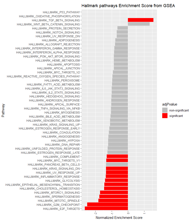
#__________bar plot _______________#
# Plot the normalized enrichment scores.
#Color the bar indicating whether or not the pathway was significant:
fgseaResTidy$adjPvalue <- ifelse(fgseaResTidy$padj <= 0.05, "significant", "non-significant")
cols <- c("non-significant" = "grey", "significant" = "red")
ggplot(fgseaResTidy, aes(reorder(pathway, NES), NES, fill = adjPvalue)) +
geom_col() +
scale_fill_manual(values = cols) +
theme(axis.text.x = element_text(angle = 90, vjust = 0.5, hjust=1)) +
coord_flip() +
labs(x="Pathway", y="Normalized Enrichment Score",
title="Hallmark pathways Enrichment Score from GSEA")
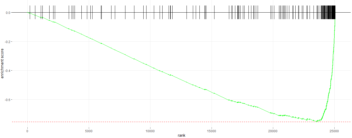
#__________Enrichment  Plot_______#
# Enrichment plot for E2F target gene set
plotEnrichment(pathway = pathways.hallmark[["HALLMARK_E2F_TARGETS"]], ranks)
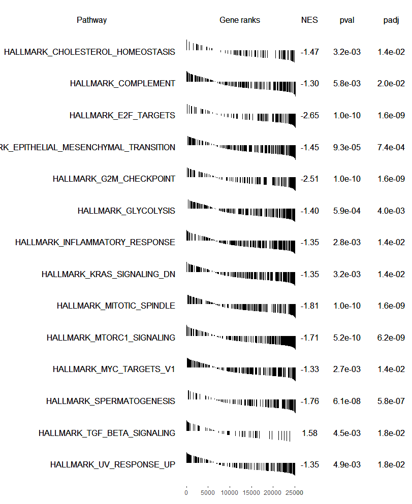
plotGseaTable(pathways.hallmark[fgseaRes$pathway[fgseaRes$padj < 0.05]], ranks, fgseaRes,
                gseaParam=0.5)
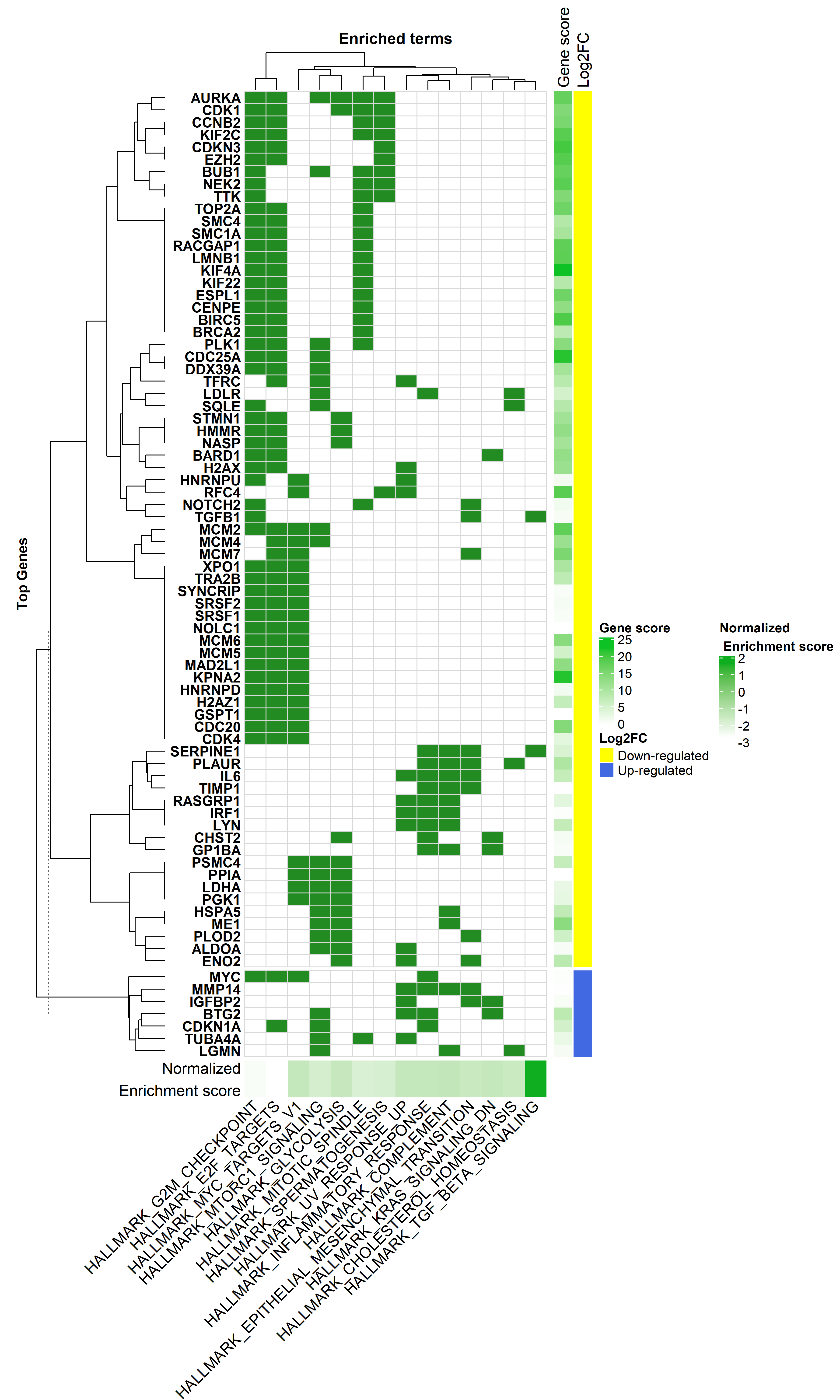
#________ Heatmap Plot_____________#
# pathways with significant enrichment score
sig.path <- fgseaResTidy$pathway[fgseaResTidy$adjPvalue == "significant"]
sig.gen <- unique(na.omit(gene.in.pathway$SYMBOL[gene.in.pathway$pathway %in% sig.path]))

### create a new data-frame that has '1' for when a gene is part of a term, and '0' when not
h.dat <- dcast(gene.in.pathway[, c(1,2)], SYMBOL~pathway)
rownames(h.dat) <- h.dat$SYMBOL
h.dat <- h.dat[, -1]

h.dat <- h.dat[rownames(h.dat) %in% sig.gen, ]
h.dat <- h.dat[, colnames(h.dat) %in% sig.path]

# keep those genes with 3  or more occurnes
table(data.frame(rowSums(h.dat)))

h.dat <- h.dat[data.frame(rowSums(h.dat)) >= 3, ]

#
topTable <- res[res$SYMBOL %in% rownames(h.dat), ]
rownames(topTable) <- topTable$SYMBOL
# match the order of rownames in toptable with that of h.dat
topTableAligned <- topTable[which(rownames(topTable) %in% rownames(h.dat)),]
topTableAligned <- topTableAligned[match(rownames(h.dat), rownames(topTableAligned)),]
all(rownames(topTableAligned) == rownames(h.dat))

# colour bar for -log10(adjusted p-value) for sig.genes
dfMinusLog10FDRGenes <- data.frame(-log10(
 topTableAligned[which(rownames(topTableAligned) %in% rownames(h.dat)), 'padj']))
dfMinusLog10FDRGenes[dfMinusLog10FDRGenes == 'Inf'] <- 0

# colour bar for fold changes for sigGenes
dfFoldChangeGenes <- data.frame(
 topTableAligned[which(rownames(topTableAligned) %in% rownames(h.dat)), 'log2FoldChange'])

# merge both
dfGeneAnno <- data.frame(dfMinusLog10FDRGenes, dfFoldChangeGenes)
colnames(dfGeneAnno) <- c('Gene score', 'Log2FC')
dfGeneAnno[,2] <- ifelse(dfGeneAnno$Log2FC > 0, 'Up-regulated',
                        ifelse(dfGeneAnno$Log2FC < 0, 'Down-regulated', 'Unchanged'))
colours <- list(
 'Log2FC' = c('Up-regulated' = 'royalblue', 'Down-regulated' = 'yellow'))
haGenes <- rowAnnotation(
 df = dfGeneAnno,
 col = colours,
 width = unit(1,'cm'),
 annotation_name_side = 'top')

# Now a separate color bar for the GSEA enrichment padj. This will
# also contain the enriched term names via annot_text()

# colour bar for enrichment score from fgsea results
dfEnrichment <- fgseaRes[, c("pathway", "NES")]
dfEnrichment <- dfEnrichment[dfEnrichment$pathway %in% colnames(h.dat)]
dd <- dfEnrichment$pathway
dfEnrichment <- dfEnrichment[, -1]
rownames(dfEnrichment) <- dd
colnames(dfEnrichment) <- 'Normalized\n Enrichment score'
haTerms <- HeatmapAnnotation(
 df = dfEnrichment,
 Term = anno_text(
   colnames(h.dat),
   rot = 45,
   just = 'right',
   gp = gpar(fontsize = 12)),
 annotation_height = unit.c(unit(1, 'cm'), unit(8, 'cm')),
 annotation_name_side = 'left')
# now generate the heatmap
hmapGSEA <- Heatmap(h.dat,
                   name = 'GSEA hallmark pathways enrichment',
                   split = dfGeneAnno[,2],
                   col = c('0' = 'white', '1' = 'forestgreen'),
                   rect_gp = gpar(col = 'grey85'),
                   cluster_rows = TRUE,
                   show_row_dend = TRUE,
                   row_title = 'Top Genes',
                   row_title_side = 'left',
                   row_title_gp = gpar(fontsize = 11, fontface = 'bold'),
                   row_title_rot = 90,
                   show_row_names = TRUE,
                   row_names_gp = gpar(fontsize = 11, fontface = 'bold'),
                   row_names_side = 'left',
                   row_dend_width = unit(35, 'mm'),
                   cluster_columns = TRUE,
                   show_column_dend = TRUE,
                   column_title = 'Enriched terms',
                   column_title_side = 'top',
                   column_title_gp = gpar(fontsize = 12, fontface = 'bold'),
                   column_title_rot = 0,
                   show_column_names = FALSE,
                   show_heatmap_legend = FALSE,
                   clustering_distance_columns = 'euclidean',
                   clustering_method_columns = 'ward.D2',
                   clustering_distance_rows = 'euclidean',
                   clustering_method_rows = 'ward.D2',
                   bottom_annotation = haTerms)

tiff("GSEA_enrichment_2.tiff", units="in", width=13, height=22, res=400)
draw(hmapGSEA + haGenes,
    heatmap_legend_side = 'right',
    annotation_legend_side = 'right')
dev.off()
Refs:
1- clusterProfiler: universal enrichment tool for functional and comparative study
2- Fast Gene Set Enrichment Analysis
3- Gene set enrichment analysis: A knowledge-based approach for interpreting genome-wide expression profiles
4- DAVID Bioinformatics Resources 6.8
5- DESeq results in pathways in 60 Seconds with the fgsea package
6- Rank-rank hypergeometric overlap: identification of statistically significant overlap between gene-expression signatures
7- Clustering of DAVID gene enrichment results from gene expression studies by Kevin Blighe.
Please correct me if I'm wrong but I don't think that you need
if you are combining
as it treats every SYMBOL as a grouping variable anyway and will always return the mean value for every repetitive.
Nice catch! you right, since
group_byis going to consider unique values no need anymore to usedistinct.Thank you very much for this tutorial. Just one question, when I run
I'm getting the following message:
Do you what this could be?
Thanks
Hi @brunobsouzaa, This error is new to me.These post may be helpful:
1- https://stackoverflow.com/questions/51986674/mclapply-sendmaster-error-only-with-rscript
2- https://r.789695.n4.nabble.com/error-in-parallel-sendMaster-td4760382.html
Thank you very much for the links... After a deep inspection, it seems that it's just a warning message. Data looks ok!
Thanks for the very nice tutorial. I was wondering what modification needs to be done for a GSEA tool (developed for microarray) to use the RNA-seq data?
None, GSEA takes ranked gene lists, no matter where they come from.
Above mentioned "the original methodology was designed to work on microarray but later modification made it suitable for RNA-seq also" so I am curious :)
I use
fgseanot the Broad version, but as said (and in my understanding) it takes ranked gene lists no matter where it comes from. I even use it for ATAC-seq to compare peak profiles across datasets. After all the GSEA is just a permutation-based test to check whether observed distributions of a set of genes (or whatever you rank and define as "set") along a ranked list are due to chance or not.@I0110 ;By design GSEA ranks genes in an expression matrix while usually RNA-seq analysis output is a pre-ranked list e.g DESeq2 output may be ranked by the Wald statistics. However in its current release its fine even to plug normalized (e.g. TMM or geometric mean) RNA-seq expression matrix in the original GSEA method.
Please check this wiki post to see what kind of modification they made on the GSEA to make it siutable for RNA-seq data also.
Hi,
I am not sure what I am doing wrong but I keep getting this error when trying to generate the heatmap. I have gone back into my code to see where it could be going wrong but I am not sure what it is referring to.
Hi,
Unless you mention your code used, it will be hard to suggest a solution.
I think I figured it out. My matrix had more that 0 or 1 for a gene count so it couldn't properly color the levels.
Hi, what did you change to fix the issue?
Hello!
I'm sorry if this isn't the right place to ask this -- but for GSEA, can someone explain in detail how to interpret the heat map in the figure in the PNAS paper?
https://www.pnas.org/content/pnas/102/43/15545/F1.large.jpg?width=800&height=600&carousel=1
The heatmap shows the genes arranged by expression fold change between
AandBin decreasing order.Thanks, friend. The colors of the heatmap are what I'm confused about. I read "expression values are represented as colors, where the range of colors (red, pink, light blue, dark blue) shows the range of expression values (high, moderate, low, lowest)." but are the genes being ranked from highest to lowest down the list or are they being ranked from highest to lowest across the list?
And in this picture, are you seeing that there are very low (dark blue), some very high (red), and some moderate (pink) levels of expression throughout all the genes in the entire gene set (from A and B)? Or am I visualizing this incorrectly? Lastly, is this showing by level of expression of the overall genes, or are these colors directly related to the ones at the top (A being red, B being blue)? If it's the former, how do we separate in this picture which genes belong to A and which genes belong to B? I think that's where my confusion is. Thanks!
Hi! When I run this part of the commands to prepare the data for the heatmap:
When I inspect h.dat variable, I get this:
I was expecting as explained in this tutorial "a new data-frame that has '1' for when a gene is part of a term, and '0' when not". What am I missing? Eventually if I follow the commands, I get the following error:
So I guess I am missing something somewhere.
Adding this should work:
Sorry if it sounds naive of me but how to make this tutorial work for normalized sequence data?
Basically you would need to replace the differential analysis part with something that accepts normalized data. That could be the limma-trend pipeline (see limma manual at Bioconductor), as input using the normalized data on log2 scale. From there on it's similar. Please open a new question for details, presenting which data you have, what you tried and where the obstacles are.
Hi all,
I am receiving this warning
I looked through my data there shouldn't be any ties or even duplicates in my L2FC.
Any suggestions?
It's not trolling you. There are ties. Use a different ranking metric that has no ties or ignore as 3% is not much.
How would I rank the following using the newly calculate parameters?
Would I change the following stats=ranks to stats = logP?