Tutorial:Create Oncoprint with ggplot2

Question

[Yun]

This tutorial makes use of the ggalign package.

The full tutorials for ggalign package deposited here: https://yunuuuu.github.io/ggalign/dev/.

In this tutorial, I will demonstrate the use of the ggalign to create an oncoprint (waterfall). We will use data from maftools package.

# load data from `maftools`
laml.maf <- system.file("extdata", "tcga_laml.maf.gz", package = "maftools")
# clinical information containing survival information and histology. This is optional
laml.clin <- system.file("extdata", "tcga_laml_annot.tsv", package = "maftools")
laml <- maftools::read.maf(
    maf = laml.maf,
    clinicalData = laml.clin,
    verbose = FALSE
)

A basic oncoprint can be generated as follows:

library(ggalign)
# Visualizing the Top 20 Genes
ggoncoplot(laml, n_top = 20)

You can then utilize the ggplot2 scales and theme to customize it:

ggoncoplot(laml, n_top = 20) +
    scale_fill_brewer(palette = "Dark2", na.translate = FALSE) +
    theme_no_axes("x")

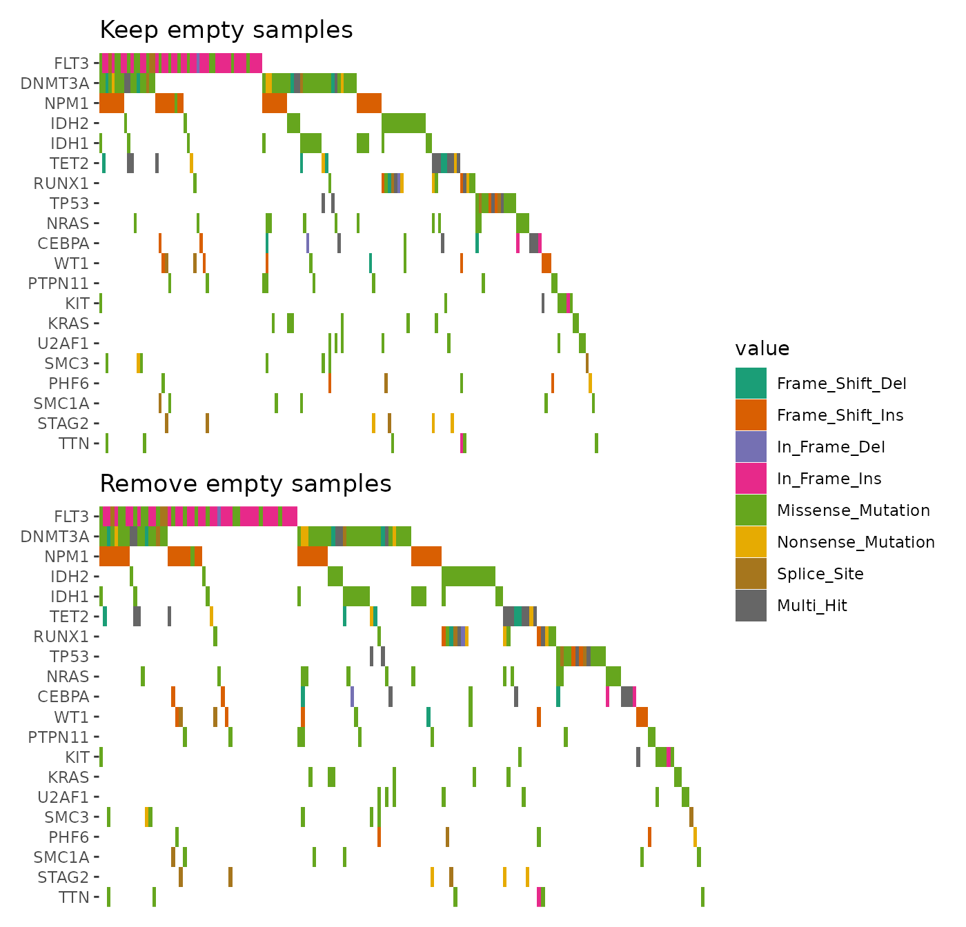
When multiple alterations occur in the same sample and gene, they are combined into a single value, "Multi_Hit", by default. To visualize these alterations separately, you can set collapse_vars = FALSE. However, doing so can lead to overlapping alterations within the same cell, making the visualization cluttered and hard to interpret.

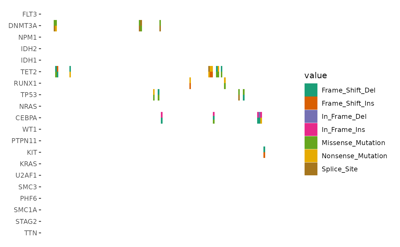
In such cases, disabling the default filling and defining a custom heatmap layer with geom_subtile() is more effective. This function subdivides each cell into smaller rectangles, allowing the distinct alterations to be clearly displayed.

Note: the Multi_Hit from last figure has been splitted into multiple tiles:

ggoncoplot(laml, n_top = 20, collapse_vars = FALSE, filling = FALSE) +
    geom_subtile(aes(fill = value), direction = "vertical") +
    scale_fill_brewer(palette = "Dark2", na.translate = FALSE) +
    theme_no_axes("x")

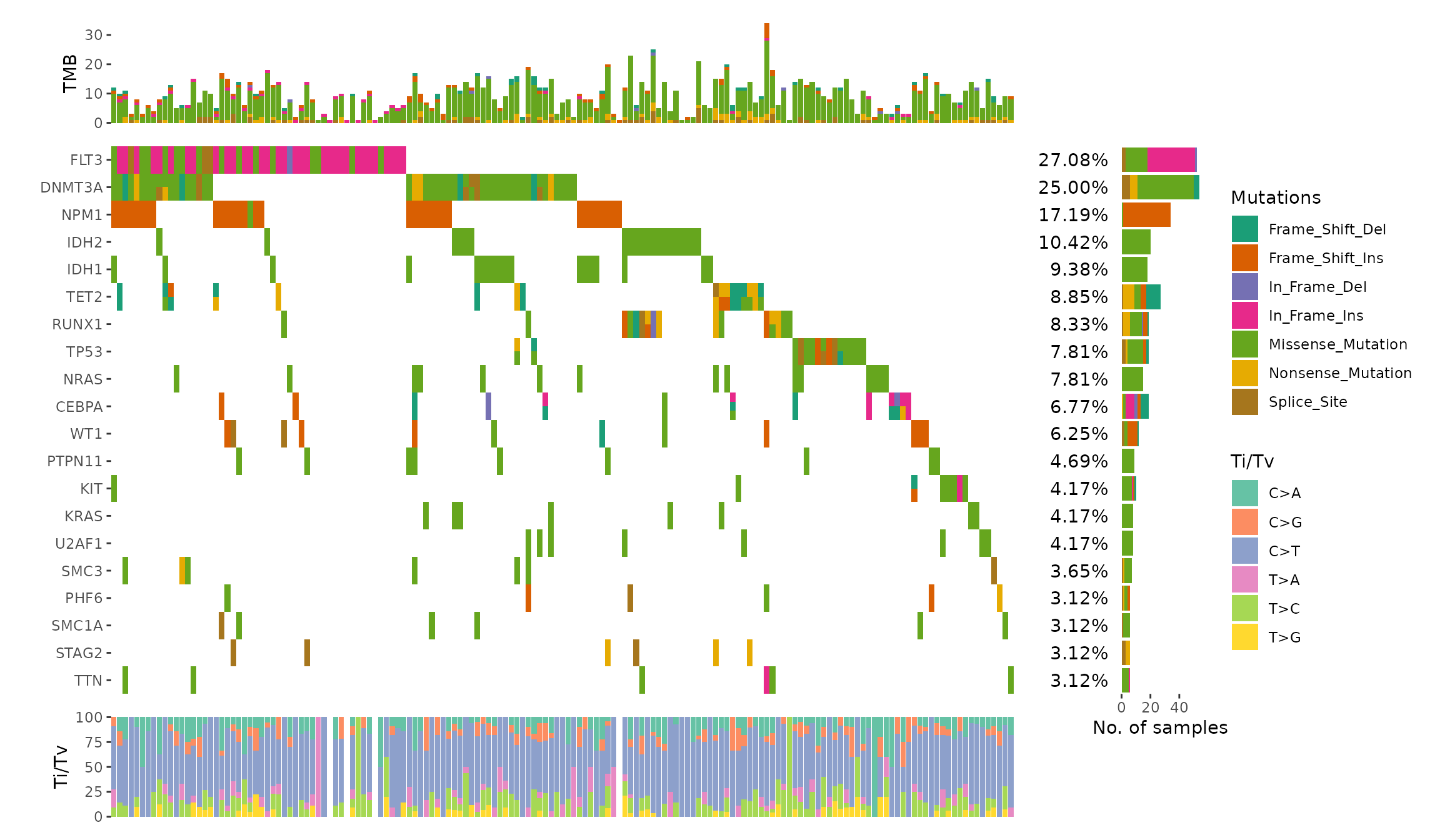
The internal will parse the MAF object and extract following informations:

• gene_summary: gene summary informations.
• sample_summary: sample summary informations.
• sample_anno: sample clinical informations.
• n_genes: Total of genes.
• n_samples: Total of samples.
• titv: A list of data.frames with Transitions and Transversions summary.

We can utilize ggalign_attr to extract the data.

ggoncoplot(laml, n_top = 20, collapse_vars = FALSE, filling = FALSE) +
    geom_subtile(aes(fill = value), direction = "vertical") +
    theme_no_axes("x") +
    # since legends from geom_tile (oncoPrint body) and `geom_bar`
    # is different, though both looks like the same, the internal
    # won't merge the legends. we remove the legends of oncoPrint body
    guides(fill = "none") +
    # add top annotation
    anno_top(size = 0.2) +
    ggalign(data = function(data) {
        data <- ggalign_attr(data, "sample_summary")
        as.matrix(data[2:(ncol(data) - 1L)])
    }) +
    geom_bar(aes(.x, value, fill = .column_names),
        stat = "identity"
    ) +
    ylab("TMB") +
    # add right annotation
    anno_right(size = 0.2) -
    # remove bottom spaces of the right annotation when aligning
    plot_align(free_spaces = "b") +
    # add the text percent for the alterated samples in the right annotation
    ggalign(data = function(data) {
        ggalign_attr(data, "gene_summary")$AlteredSamples /
            ggalign_attr(data, "n_samples")
    }) +
    geom_text(aes(1, label = scales::label_percent()(value)), hjust = 1) +
    scale_x_continuous(
        expand = expansion(),
        name = NULL, breaks = NULL,
        limits = c(0, 1)
    ) +
    theme(plot.margin = margin()) +
    # add the bar plot in the right annotation
    ggalign(data = function(data) {
        data <- ggalign_attr(data, "gene_summary")
        as.matrix(data[2:8])
    }) +
    geom_bar(aes(value, fill = .column_names),
        stat = "identity",
        orientation = "y"
    ) +
    xlab("No. of samples") -
    # we apply the scale mapping to the top and right annotation: `position = "tr"`
    # and the main plot: `main = TRUE`
    with_quad(
        scale_fill_brewer("Mutations",
            palette = "Dark2", na.translate = FALSE
        ),
        position = "tr",
        main = TRUE
    ) +
    # add bottom annotation
    anno_bottom(size = 0.2) +
    # add bar plot in the bottom annotation
    ggalign(data = function(data) {
        data <- ggalign_attr(data, "titv")$fraction.contribution
        as.matrix(data[2:7])
    }) +
    geom_bar(aes(y = value, fill = .column_names), stat = "identity") +
    ylab("Ti/Tv") +
    scale_fill_brewer("Ti/Tv", palette = "Set2")

geom_subtile() often suffices for most scenarios. However, if you require a strategy similar to that of ComplexHeatmap, consider using geom_draw(), which offers greater flexibility for complex customizations. It is a ggplot2 layer function but do the same things of ComplexHeatmap layer_fun. For more details, please see https://yunuuuu.github.io/ggalign/dev/articles/oncoplot.html

[yura.grabovska]

What are the pros/cons of using this over ComplexHeatmap?

[Yun]

Hi, @yura.grabovska Thank you for your response.

Pros of ggalign: One of the biggest strengths of ggalign is its seamless integration with ggplot2. This brings several benefits:

1. Access to ggplot2 Geoms: Users can take advantage of a rich ecosystem of ggplot2 extensions, like ggpattern, ggbeeswarm, ggsignif et al. ggalign also provide some useful geoms like a heatmap pie charts:

   set.seed(123)
   ggheatmap(matrix(runif(360L), nrow = 20L), filling = NULL) +
   geom_pie(aes(angle = value * 360, fill = value))
   

   

   1. Access to the rich of color scales (rich of palette).

   2. Automatic Legends: Unlike ComplexHeatmap, which often requires manual legend creation, ggplot2 handles this automatically.

   3. Dendrogram can be easily customized and colored, I have attached the full data (both dendrogram node and dendrogram edge) into the object (align_dendrogram()), if you want to color notes or branches, just add a new geom:

set.seed(123)
small_mat <- matrix(rnorm(81), nrow = 9)
rownames(small_mat) <- paste0("row", seq_len(nrow(small_mat)))
colnames(small_mat) <- paste0("column", seq_len(ncol(small_mat)))
ggheatmap(small_mat) +
    anno_top() +
    align_dendro(aes(color = branch), k = 3) +
    geom_point(aes(color = branch, y = y))

1. Simplified Alignment with Other ggplot2 Plots is straightforward by panel area.

2. Lower Learning Curve, For those familiar with ggplot2, ggalign requires little extra effort, as it avoids reliance on grid syntax.

Developer Insights: We've designed ggalign with flexibility in mind, separating layout control from the main function. Currently, four key layout functions are available:

• align_group: Group and align plots based on categorical factors.
• align_order: Reorder layout observations based on statistical weights or allows for manual reordering based on user-defined ordering index.
• align_kmeans: Group observations by k-means clustering results.
• align_dendro: Align plots according to hierarchical clustering or dendrograms.

Adding new layout control methods is simple—just create a new Align object as a ggproto extension, following the conventions of ggplot2.

Moreover, extending ggalign with other object types is straightforward. Developers can define new fortify_matrix or fortify_data_frame methods to integrate their objects. For instance, ggalign currently supports MAF and GISTIC objects from the maftools package via built-in fortify_matrix methods.

Cons: Fewer Built-In Annotations: May require additional coding for specific annotations or customization compared to the extensive built-in annotation function in ComplexHeatmap. But I'm planning to wrap some common plot types for user convenience.