Hi
I'm using VarScan to call CNVs. I've generated raw, called, adjusted GC content and the segmented file of Copy Number. But
I don't know the code that how to plot the CNVs using R? Can anybody share the code? And which file that I've generated using VarScan should I use?
CNVkit has some nice visualizations that are pretty easy to use. You may have to do some finagling to get your files to match their format, but it shouldn't be too difficult.
If you're dead set on an R option, pureCN and DNAcopy both have some plotting functions, though again, you may have to tweak your files slightly to match their formats.
Without showing us your files or what plots you want to actually make, it's difficult to give a more specific answer.
Please try to post comments as comments rather than answers, as it makes conversation easier to follow. You can also always add more information to your original question by editing it. Additionally, please use the code formatting button (the one with 1's and 0's) to format code so that it's readable.
The last figure is analogous to CNVkit's scatter command. The other two will require a bit of thought and manual manipulation on your part. The first will require you to average the log2 ratio at each bin for all your samples, then it's basically just a bar plot split by chromosomes. The second will require you to have gain/loss at each bin for each sample and simply calculate the percentage of each for each bin. Both of those plots, maybe minus the annotation bar at the bottom, could be easily done in ggplot2. The karyotype addition at the bottom is something you'd have to figure out on your own.
The first plot better be done via GISTIC 2.0 (using results from VarScan). The 2nd plot does not look informative to me. The third plot may be done via plot function in R sample by sample, however, you'll need to prepare a chromosome structure yourself. As for me, I like visualizations from FACETS since it gives MUCH more insights into the tumor structure. I like visualizations from my tool more, but if you want something quick - use FACETS.
The first plot can't be replicated from GISTIC2, though you're correct that it creates something that's analogous to it. Definitely worth a shot. Hadn't heard of FACETS before, documentation looks kind of sparse, but will have to give it a shot some time.
Honestly, I can not say that I fully understand if the first plot is a multi-sample one or it is a single sample. If it is multi-sample - GISTIC IMHO gives a more meaningful plot of significant pikes. If it is one-sample - then why, FACETS-like plots would be better. Personally, I prefer this plots (they are easier for me to understand than even FACETS one) , but have to admit - it is easier and faster to run FACETS. And it works quite good.
The first one differs slightly from GISTIC in that GISTIC really is focused on minimal common regions (MCRs), which are the spikes in the GISTIC plot. It's really meant for identifying recurrent focal CNAs and their potential driver genes. The first plot here summarizes not only focal changes, but broad changes as well by averaging the log2 ratios across multiple samples.
If just highlighting recurrently amplified/deleted genes in their genomic context is what you're after, either works, but the plot here also serves to show a general idea of the CNA changes across all samples.
Mind explaining your top and bottom plots here? It's not totally clear what they're showing.
Oh, thanks. I am not good in reading manuals when there are deadlines and I was thinking where my recurrent aneuploidies disappeared in my cancer samples in GISTIC - now I know. For me it is still difficult to infer something from the first plot (it is a sum of all samples, but there are sub-groups almost always), but I get the logic.
Yeap, the top plot shows B-allele frequency of normally heterozygous SNVs - everything that deviates from 0.5 (the y-axis is from 0 to 1) indicates a presence of CNA. The bottom plot shows the allelic decomposition. Two bold horizontal lines for each segment - integer copy-numbers of each segment (for both alleles). When one bold line drops to 0 - it is a deletion of the minor allele. The color indicates a Cancer Cell Fraction (lighter color = smaller sub-clone). In general, I've tried to do my best to explain it here - https://github.com/imgag/ClinCNV/blob/master/doc/somatic_CNA_analysis.md#cnas-visualization-plots - and looking for a criticism, if it is clearly explained.


Please try to post comments as comments rather than answers, as it makes conversation easier to follow. You can also always add more information to your original question by editing it. Additionally, please use the code formatting button (the one with 1's and 0's) to format code so that it's readable.
The last figure is analogous to CNVkit's
scattercommand. The other two will require a bit of thought and manual manipulation on your part. The first will require you to average the log2 ratio at each bin for all your samples, then it's basically just a bar plot split by chromosomes. The second will require you to have gain/loss at each bin for each sample and simply calculate the percentage of each for each bin. Both of those plots, maybe minus the annotation bar at the bottom, could be easily done in ggplot2. The karyotype addition at the bottom is something you'd have to figure out on your own.The first plot better be done via GISTIC 2.0 (using results from VarScan). The 2nd plot does not look informative to me. The third plot may be done via plot function in R sample by sample, however, you'll need to prepare a chromosome structure yourself. As for me, I like visualizations from FACETS since it gives MUCH more insights into the tumor structure. I like visualizations from my tool more, but if you want something quick - use FACETS.
The first plot can't be replicated from GISTIC2, though you're correct that it creates something that's analogous to it. Definitely worth a shot. Hadn't heard of FACETS before, documentation looks kind of sparse, but will have to give it a shot some time.
Honestly, I can not say that I fully understand if the first plot is a multi-sample one or it is a single sample. If it is multi-sample - GISTIC IMHO gives a more meaningful plot of significant pikes. If it is one-sample - then why, FACETS-like plots would be better. Personally, I prefer this plots (they are easier for me to understand than even FACETS one)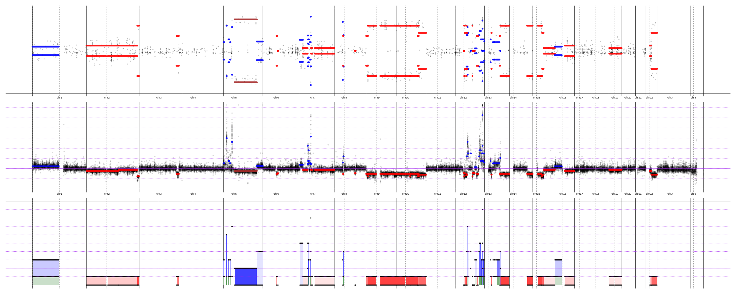 , but have to admit - it is easier and faster to run FACETS. And it works quite good.
The first one differs slightly from GISTIC in that GISTIC really is focused on minimal common regions (MCRs), which are the spikes in the GISTIC plot. It's really meant for identifying recurrent focal CNAs and their potential driver genes. The first plot here summarizes not only focal changes, but broad changes as well by averaging the log2 ratios across multiple samples.
If just highlighting recurrently amplified/deleted genes in their genomic context is what you're after, either works, but the plot here also serves to show a general idea of the CNA changes across all samples.
Mind explaining your top and bottom plots here? It's not totally clear what they're showing.
Oh, thanks. I am not good in reading manuals when there are deadlines and I was thinking where my recurrent aneuploidies disappeared in my cancer samples in GISTIC - now I know. For me it is still difficult to infer something from the first plot (it is a sum of all samples, but there are sub-groups almost always), but I get the logic.
Yeap, the top plot shows B-allele frequency of normally heterozygous SNVs - everything that deviates from 0.5 (the y-axis is from 0 to 1) indicates a presence of CNA. The bottom plot shows the allelic decomposition. Two bold horizontal lines for each segment - integer copy-numbers of each segment (for both alleles). When one bold line drops to 0 - it is a deletion of the minor allele. The color indicates a Cancer Cell Fraction (lighter color = smaller sub-clone). In general, I've tried to do my best to explain it here - https://github.com/imgag/ClinCNV/blob/master/doc/somatic_CNA_analysis.md#cnas-visualization-plots - and looking for a criticism, if it is clearly explained.