You can use karyoploteR to create a plot similar to a manhattan plot and using any genome.
To create such plot you should first create an empty plot following these instructions and giving it a GRanges or a BED file with the chromosome sizes of C. Albicans (you can get them from this table.
After that, you just need to plot the points representing your snps using the kpPoints function. You can follow the examples at the tutorial or at the rainfall plot example, although the second one is a bit more complex.
Don't forget to use plot.type=4 as in the rainfall plot example to give it a more traditional manhattan plot look and feel.
EDIT:
Following the comments, I'm here is some code to create a basic plot.
karyoploteR needs chromosome information to work, so I'll assume the data is in a file with the following format:
Chr Pos Frequency
chr1A   15305   4
chr1A   168836  7
chr1A   515835  1
chr1A   515850  3
chr1A   837522  4
chr1A   842901  7
with the columns separated by tabs.
library(karyoploteR)

#Read the data from a file in the same directory called "SNPS.txt"
snps <- read.table(file = "SNPs.txt", sep = "\t", header=TRUE, stringsAsFactors = FALSE)

#Create a GRanges object with the chromosomes and length found at http://www.candidagenome.org/cache/C_albicans_SC5314_genomeSnapshot.html
calbicans.genome <- toGRanges(data.frame(chr=c("chr1A", "chr1B", "chr2A", "chr2B", "chr3A", "chr3B", "chr4A", "chr4B", "chr5A", "chr5B", "chr6A", "chr6B", "chr7A", "chr7B", "chrRA", "chrRB"),
                    start=rep(1, 16),
                    end=c(3188341, 3188396, 2231883, 2231750, 1799298, 1799271, 1603259, 1603311, 1190869, 1190991, 1033292, 1033212, 949580, 949611, 2286237, 2285697)))

#Create the plot
kp <- plotKaryotype(genome=calbicans.genome, plot.type=4, ideogram.plotter = NULL, labels.plotter = NULL)
kpAddCytobandsAsLine(kp)
kpAddChromosomeNames(kp, srt=45)

max.freq <- max(snps$Frequency)

kpAddLabels(kp, "SNP Frequency", srt=90, pos=3)
kpAxis(kp, ymin = 0, ymax=max.freq)
kpPoints(kp, chr=snps$Chr, x=snps$Pos, y=snps$Frequency, ymin=0, ymax=max.freq)
You can ajdust multiple additional parameters then the size of the points and their colors. the margins... You can find more information on how to do it in the documentation.
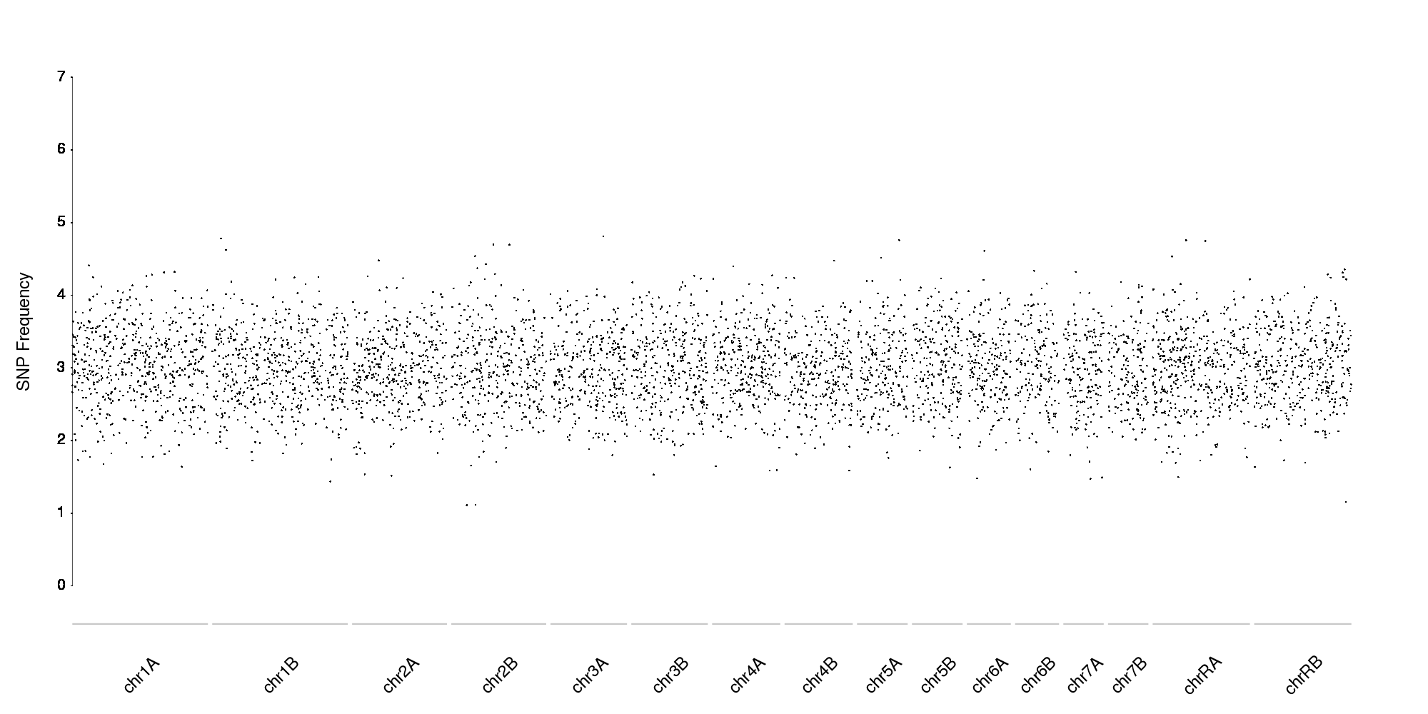
With more data points (in this case, random data) it would look like this


Thanks for the really detailed reply! This really helped me. However, I don't quite get the instructions for the tutorial to create a simple plot. I don't quite understand the code and how to manipulate the code to manually add my data. How does the program acquire the data for each of the 23 data points?
Thanks so much! You've already been of great help!
Just to clarify my question, I have no clue how to plot an ideogram by loading my own custom data of SNP frequencies.
Hi nattzy94,
The data in the example is randomly created with
x <- 1:23*10e6andy <- rnorm(23, mean=0.5, sd=0.25). In your case you would probably read it from a file with the data about your snps (position and frequency). If you can paste here the first lines of your data file I can try to help you with that.Thanks so much. I'm new to R so really appreciate the help!
Pos...........Frequency
151305.........4
168836.........7
515835.........1
515850.........3
837522.........4
842901.........7
Realized I did not provide the chromosome information. Just assume it is all chr 1. Also, I do not need to plot chromosome features. Thanks for your time!
Hi Bernatgel,
Have you had a chance to look at the data? I can modify the data if it is not suitable.
I edited the original answer to include some code
ok. Thanks so much bernatgel!
ok. Thanks so much bernatgel!