Coverage plot of a complete genome

Question

[frymor2]

In a paper I was reading i have found the attached image. It shows the duplication of specific chromosomes in different yeast strains after treatment with antibiotics.

I was wondering how can one plot the whole genome in such a way? Are there any tools or R packages to get such a result?

thanks

[German.M.Demidov]

tbh, it looks like a CNV caller worked here =) the plots looks too uniform - which means they were likely GC/library size normalized before plotting

or it is a rolling median across the coverage precalculated in some windows (e.g. 50kbps)

[scheitelt]

yes, This is true, but it doesn't really answer the question. The question was how this plot was done. can some please help me too?

[German.M.Demidov]

You can calculate the coverage per some window, smooth it with rolling median and plot in R - this is what I would do

Answer 1

[Pierre Lindenbaum]

I wrote http://lindenb.github.io/jvarkit/WGSCoveragePlotter.html

[frymor2]

Thanks Pierre, this looks good. Is it possible to use a bam file with multiple read groups as an input here?

[Pierre Lindenbaum]

you meant that there is only more that one sample ? everything would be merged here, but I can add an option to only select a defined sample.

[frymor2]

What I meant is, if there is a possibility to take a bam file with multiple samples, defined by separate read groups and use it as an input. I have a concatenated bam files I have merged from several single samples, for several reasons. Now I would like to plot this bam file, but to get the coverage separated by the single samples (e.g marked by the read groups). This should be something like the the facet_wrap in the R command ggplot. One row should represent one read group instead of a whole bam file.

Would this be possible?

[Pierre Lindenbaum]

I've just added an option --samples http://lindenb.github.io/jvarkit/WGSCoveragePlotter.html

[frymor2]

thanks, I'll give it a go as soon as as possible and come back to you

Answer 2

[William]

Hi!

You can use also check out the python program bam2plot, which I have developed. Install via pip install bam2plot, and run:

bam2plot my_bam.bam

It produces one png and one svg for each reference (e.g. chromosome) in the bam file.

Check it out here: https://github.com/willros/bam2plot

Regards, William

Answer 3

[cmdcolin]

I think that it can be useful to learn to plot this using R, from code. there is a crucial sort of "realization" i had with this is that you create a "cumulative base pair" transformation, so if all your chromosomes are 1000bp long, then you make chr1 occupy the number space 1-1000, then then chr2 is 1001-2000, chr3 from 2001-3000. there are some nice one liners in R that do this, and afterwards, you can tell R to draw the chromosome labels at these given coordinates.

I created simulated reads for yeast, then calculated coverage with mosdepth (https://github.com/brentp/mosdepth), and then loaded the resulting coverage into R with simple read.table commands and plotted with ggplot2

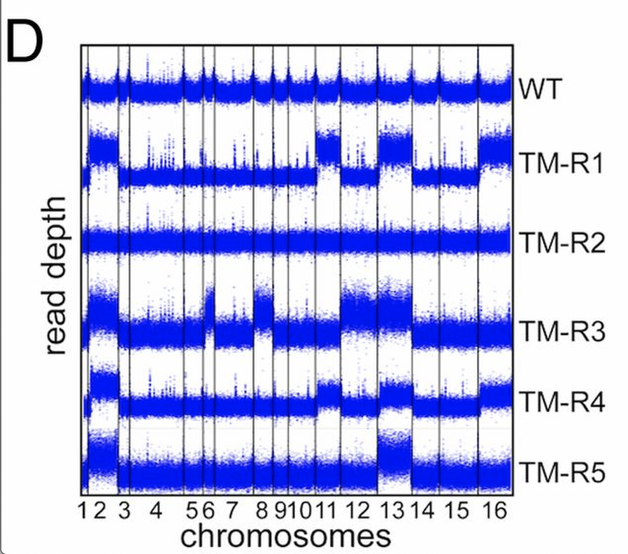
Here is the "setup"

Create a "quickalign" script that aligns paired end reads and outputs mosdepth coverage

the quickalign script

#!/bin/bash
# quickalign_paired.sh ref.fa 1.fq 2.fq out.cram
# produces out.cram and out.regions.bed.gz containing 100bp window mosdepth coverage
# based on http://www.htslib.org/workflow/fastq.html for the one-liner fastq-to-cram
samtools faidx $1
minimap2 -t 8 -a -x sr "$1" "$2" "$3"  | \
samtools fixmate -u -m - - | \
samtools sort -u -@2 - | \
samtools markdup -@8 --reference "$1" - --write-index "$4"


mosdepth $4 -b 100 -f $1 $4

Run quickalign over some simulated reads, generated by wgsim

wgsim GCF_000146045.2_R64_genomic.fna a1.fq a2.fq
wgsim GCF_000146045.2_R64_genomic.fna b1.fq b2.fq
wgsim GCF_000146045.2_R64_genomic.fna c1.fq c2.fq
quickalign_paired.sh GCF_000146045.2_R64_genomic.fna a1.fq a2.fq out1.cram
quickalign_paired.sh GCF_000146045.2_R64_genomic.fna b1.fq b2.fq out2.cram
quickalign_paired.sh GCF_000146045.2_R64_genomic.fna c1.fq c2.fq out3.cram

R session for plotting coverage

library(tidyverse)
x1=read.table('out1.cram.regions.bed.gz')
x2=read.table('out2.cram.regions.bed.gz')
x3=read.table('out3.cram.regions.bed.gz')
colnames(x1)<-c("chr","start","end","score")
colnames(x2)<-c("chr","start","end","score")
colnames(x3)<-c("chr","start","end","score")
chrom_sizes=read.table('GCF_000146045.2_R64_genomic.fna.fai')
colnames(chrom_sizes)<-c("chr","size")
chrom_sizes=chrom_sizes[,c(1,2)]

data_cum <- chrom_sizes %>%
  group_by(chr) %>%
  summarise(max_bp = max(size)) %>%
  arrange(-max_bp) %>%
  mutate(bp_add = lag(cumsum(as.numeric(max_bp)), default = 0))

process <- function(df) {
  df %>%
    inner_join(data_cum, by = "chr") %>%
    mutate(bp_start_cum = start + bp_add) %>%
    mutate(bp_end_cum = end + bp_add)
}
data1 <- process(x1)
data2 <- process(x2)
data3 <- process(x3)
data1$id <- "id1" #labels used for each row in the plot
data2$id <- "id2"
data3$id <- "id3"
df <- rbind(data1, data2, data3)

axis_set <- data_cum %>%
  group_by(chr) %>%
  mutate(center = bp_add)

# plotting using small geom_point
p<-ggplot(data = df) +
  geom_point(aes(x=bp_start_cum, y=score),size=0.1,alpha=0.2) +
  scale_x_continuous(label = axis_set$chr, breaks = axis_set$center) +
  facet_grid(rows = vars(id)) +
  theme(
    axis.text.x = element_text(angle = 60, size = 8, vjust = 0.5),
    axis.title.x=element_blank()
  )

ggsave('out.png',width=10,height=4)

Note: I adapted some code I wrote for this answer How to create a graph that shows pairwise Fst values at single SNP loci across the all chromosomes in R